Tag: South Carolina

This is map ensures a Republican 6 to 1 delegation for the entire decade. It strenghtens Wilson’s district while creating a new Republican seat. I currently live in District 4 and am active in the redistricting process.

District 1 – Tim Scott

68% White
21% AA
7.2% Hispanic

This uses some Republican low country areas from Clyburn’s old district along with Republican Charleston and Hilton Head to create a Safe Republican district for Scott.

District 2 – Joe Wilson

73.5% White
18.1% AA
5% Hispanic

A Lexington County based district that adds some of the conservative upstate while dropping some southern counties. Adds Calhoun County from Clyburn’s old district (SC-6) and loses some Democrat areas of Columbia in Richland County. The new SC-2 then extends north to pick up parts of heavily republican Anderson and Pickens Counties from SC-3. A Safe Republican district for Wilson.

District 3 – Jeff Duncan

69.5% White
23.7% AA
4.3% Hispanic

This new SC-3 district picks up parts of Wilson’s old districts opposite Augusta (from Wilson)and western Orangeburg Country (from Clyburn), while giving up parts of upstate counties to SC-2 (Joe Wilson’s district). In addition, it maintains Duncan’s residence in the district. Safe Republican.

District 4 – Trey Gowdy

67.5% White
22.4% AA
6.6% Hispanic

Greenville County based upstate district that includes Gowdy’s Spartanburg residence and the most democratic areas of downtown Spartanburg. The new 4th also adds two counties of Spratt’s old district. The new configuration keeps SC-4 from being a Republican vote sink while still being a solid republican district. Safe Republican.

District 5 – Mick Mulvaney

69.1% White
22.8% AA
4.7% Hispanic

By adding heavily republican northern Spartanburg County, York based SC-5 is able to keep Kershaw County (stopping Vincent Shaheen from running in SC-7) and the Democratic regions of Dilon and Marlboro Counties. Divides the rest of the counties that kept reelecting Spratt to SC-4, SC-6, and the new SC-7. A Safe Republican district for Mulvaney.

District 6 – Jim Clyburn

30.9% White
62.5% AA
3.8 % Hispanic

This District gives up some low country republican areas, Calhoun and western Orangeburg counties, while picking up more of Columbia, and parts of Lee and Darlington Counties from SC-5. Also picks up parts of low country counties from SC-2, and gives up more republican areas closer to Horry County.

A genuine, quite fair Majority-Minority district now. Safe Democrat.

District 7 – New Open Seat

69.9% White
23.1% AA
4.1% Hispanic

With Horry County and the northeastern exurbs of Charleston to anchor this district, this should be safely Republican for the foreseeable future. Republicans should be very competitive even in the parts of the district outside of Horry and Ex-urban Charleston. Likely to Safe Republican.

—

Distribution of Columbia/Richland County:

Greenville/Upstate:

Charleston/Beaufort:

 —
Questions and comments are welcome.

Rhode Island doesn’t offer much for redistricting fans to sink their teeth into: it has two districts that are about equally blue, the Dems control the redistricting trifecta, and the disparity between the two districts, while not New Hampshire-close, requires only minimal boundary-shifting. Rhode Island’s target is a tiny 526,284 (only up from 524K in 2000… Rhode Island had the smallest growth, percentage-wise, of any state over the decade, putting it 2nd overall behind only Michigan, which actually lost population). If this continues, there’s the distinct possibility we could see Rhode Island reduced to one House seat come 2020. Also worth noting: Rhode Island had a lot of Hispanic growth over the decade, not quite on par with the Southwest but high for the Northeast; it went from 8.5% Hispanic to 12.4%, and Providence moved to a Hispanic plurality.

South Carolina is gaining one seat to move from six to seven; its new target based on 7 seats is 660,766 (it was 668K in 2000, so every district gained significantly over the decade). With the GOP holding the trifecta and much of the growth seeming to come among white retirees, look for the creation of one more Republican-friendly seat… with one possible wild card, that the Obama DOJ might weigh in and push for a second African-American VRA seat (theoretically possible if terribly ugly, as SSP’s crack team of freelance mapmakers have shown here). The biggest growth has come in the coastal Low Country, rather than the fiercely evangelical uplands; I’d expect Charleston and Myrtle Beach, both part of SC-01 for now, to wind up each anchoring their own districts.

West Virginia is staying at three seats for now, although it might be headed for two seats in 2020, given its slow growth and low targets; its target is 617,665, only up from 603K in 2000. The 3rd, in coal country in the southern part of the state, is losing population (though not as fast as one might suspect); the 2nd needs to shed an amount equivalent to what the 3rd needs to gain, leaving the 1st pretty stable. Much of the state’s growth is in the far east tip of the Panhandle (in the 2nd), especially Berkeley County, which serves as Washington DC’s furthest-out exurbs. Dave Wasserman, who seems to get all the good redistricting-related gossip, says that while the obvious solution (moving Mason County from the 2nd to the 3rd, and calling it a wrap) still seems likely, the Dems who control the redistricting trifecta might want to cobble together a slightly Dem-friendlier 1st along the state’s northern boundary that includes both Morgantown and the Panhandle exurbs (the only counties in the state that are getting bluer).

In my research on South Carolina’s 2010 gubernatorial election, I came upon a fascinating chart. The chart describes the number of Democrats and Republican in South Carolina’s State House of Representatives from the Civil War to the present day. The data offers a fascinating story of the Democratic Party in South Carolina, and the Deep South in general.

Here is the story:

Most individuals familiar with politics know the history of the Deep South: it seceded from the Union after President Abraham Lincoln was elected. In the resulting Civil War, it fought the hardest and suffered the most against Union forces.

Victorious Union forces were identified with the hated Republican Party, founded with the explicit goal of destroying the southern way of life by ending slavery.

Under military Union rule, the Republican Party flourished in South Carolina:

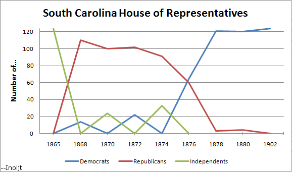
The Republican Party was the dominant political force during the Reconstruction era, as the graph above shows. During its reign in power, it enjoyed large majorities in the State House of Representatives. Its political base was the black vote, and it attempted to systemically ensure racial equality for blacks and whites. A number of blacks were elected to state and federal office; it’s probable that many of the Republicans in the State House of Representatives were black.

This enraged whites in South Carolina. When President Rutherford Hayes ended Reconstruction and withdrew federal troops, they quickly gained control of South Carolina politics. The black vote was systemically crushed, and along with it the Republican Party.

This is reflected in the graph above. In 1874 there were 91 Republicans in the State House of Representatives. By 1878 there were only three left.

This led to the next stage of South Carolina politics, the Solid South:

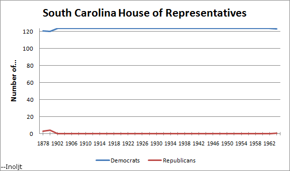
Unfortunately, Wikipedia does not have data after 1880 and before 1902. After 1902, however, Democrats enjoyed literally absolute control of the State House of Representatives. For more than half-a-century, not a single Republican in South Carolina was elected to the State House of Representatives. Democrats regularly won over 95% of the popular vote in presidential elections.

That’s a record on par with that of the Communist Party in the Soviet Union.

There are several reasons why this occurred. Democrats in South Carolina were strongest of all the Deep South states, because blacks were the majority of the population. Only Mississippi at the time also had a black-majority population.

This meant that in free and fair elections, blacks would actually have control of South Carolina politics. If a free and fair election took place in another Southern states, the Democratic Party would still probably have maintained power – since whites were a majority of the population. In fact, this is what happens in the South today, except that the roles of the two parties are switched.

This was not the case with South Carolina, and party elites were profoundly aware and afraid of this. Therefore the grip of the Democratic Party was tightest in South Carolina, of all the Solid South (South Carolina was the first state to secede from the Union for the same reason). Other Solid South states had more than zero Republicans in the state legislature. Republican presidential candidates might gain 20-40% of the vote, rather than less than 5%.

In black-majority South Carolina, the Republican Party was a far greater potential threat – and so the Democratic Party was extraordinarily judicious in repressing it.

Racism was a useful tool for South Carolina Democrats, and they were very proud racists. Controversial South Carolina Governor and Senator Benjamin Tillman, for instance, once stated that:

I have three daughters, but, so help me God, I had rather find either one of them killed by a tiger or a bear and gather up her bones and bury them, conscious that she had died in the purity of her maidenhood by a black fiend. The wild beast would only obey the instinct of nature, and we would hunt him down and kill him just as soon as possible.

Another time he commented:

Great God, that this proud government, the richest, most powerful on the  globe, should have been brought to so low a pass that a London Jew  should have been appointed its receiver to have charge of the treasury.

This was the Democratic Party of South Carolina during the Solid South.

At the end of the graph, notice that there is a little dip, just after the year 1962. This was in 1964, when the first Republican in more than half-a-century was elected to the South Carolina State House of Representatives.

He was not the last:

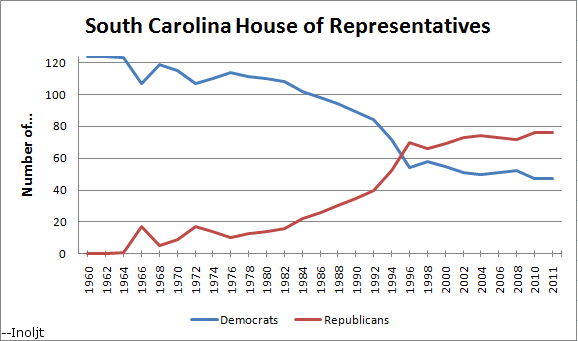
The year 1964 marked the day that Democratic President Lyndon B. Johnson pushed through the 1964 Civil Rights Act, against enormous Southern Democratic opposition.

It also marked the beginning of the end of the South Carolina Democratic Party. The Democratic Party underwent a monumental shift, from a party of white elites to a party representing black interests. In the process South Carolina whites steadily began abandoning it.

At first the decline was gradual, as the graph shows. In 1980 there were 110 Democrats in the State House of Representatives and 14 Republicans. Throughout the 80s the Democratic majority steadily declined, but in 1992 there were still 84 Democrats to 40 Republicans.

Then came 1994 and the Gingrich Revolution. The seemingly large Democratic majority collapsed like the house-of-cards it was, as South Carolina whites finally started voting for Republican statewide candidates, decades after they started doing so for Republican presidential candidates. Republicans have retained control of the state chamber ever since.

Since then the Democratic Party has declined further in the State House of Representatives. As of 2010 the number of Democratic representatives is at a 134-year low. And the floor may not have been reached. There are still probably some conservative whites who vote Democratic statewide, when their political philosophy has far more in common with the Republican Party.

Nevertheless, the modern era in South Carolina politics is still shorter than the Solid South era. Here is the entire history of the State House of Representatives:

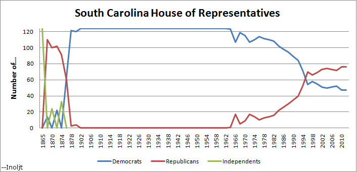
It’s a fascinating graph, and it tells a lot about South Carolina and Deep South politics.

–Inoljt, http://mypolitikal.com/

This is part of three posts analyzing the 2010 South Carolina  gubernatorial election, in which Republican Nikki Haley won a  closer-than-expected victory over Democrat Vincent Sheheen. The main  focus of these posts will be to explore whether a racial effect  accounted for Ms. Haley’s unexpected poor performance.

(Note: This is also part of a series of posts analyzing the 2010 midterm elections.)

More below.

The previous post mapped out the relationship between Democratic shifts in 2010 and white registration numbers. Here is the relevant map reposted:

The post ended by noting that “So far this analysis has been relatively light on the statistical side of things.” It included a number of maps, but did not use any raw numbers.

This post aims to draw conclusions based on those numbers.

Let’s begin by translating the picture above into a graph:

This graph maps the relationship between how white a county in South Carolina is, and how much it shifted against non-white Republican candidate Nikki Haley in 2010.

If normally-Republican whites moved against Ms. Haley due to her race, one would expect the dots to be graphed in a roughly 45-degree diagonal line; the whiter a county, the more Democratic it would shift in 2010.

Clearly this is not the case in the graph above. There are a lot of very white counties that shifted strongly against Ms. Haley – but there are also a lot of very white counties that supported her more than they did Senator John McCain.

Indeed, the whitest counties seem to spread out into two groups; one group moves strongly against Ms. Haley, another actually shifts for her. One might speculate that the former group is composed of lower-income, rural whites and the latter is composed of higher-income, metropolitan whites.

To test this theory, the previous post adjusted for income by eliminating all the counties with a median household income greater than the state median (i.e. it got rid of the rich whites). Here is what the result looked like:

There seems to be a correlation here, as the previous post noted.

Here is how the relationship looks on a graph:

The group of white counties which shifted towards Ms. Haley has disappeared. Instead, one sees a much stronger trend: the whiter the county, the more strongly it moved against non-white Republican Governor Nikki Haley.

This only happens once high-income white counties are tossed out of the analysis. High-income Republican whites were very comfortable voting for non-white Republicans; low income Republican whites were less willing.

Interestingly, this pattern is not unique to South Carolina. In Louisiana, Republican Governor Bobby Jindal – a non-white individual of Indian descent – did extremely poorly amongst rural, low-income (Republican) whites while winning landslide support amongst high-income, suburban (Republican) whites. This caused Mr. Jindal to lose in his first attempt to run for governor.

Finally, one can test whether the effect above is statistically significant, or just the result of randomness.

Here is a regression analysis run on the 2010 South Carolina gubernatorial race:

Regression analysis is something I am still not fully comfortable with, so bear this in mind as the analysis continues.

The regression attempted to use two variables – race and income – to predict whether voters would vote more Democratic in 2010. Specifically, it used the percent of white registered voters in a county and said county’s median household income.

The model states that every 10% increase in white registered voters results in a 3.65% greater Democratic shift against Ms. Haley (this is the Coefficient column at the bottom left).

More importantly, whiteness and income were statistically significant when placed together; there was a 0.1% chance that the effect of whiteness was random, and a 0.4% chance that the effect of income was random (this is the P>|t| column at the bottom center).

So the evidence is fairly strong that racially-based voting by low-income whites hurt non-white Republican Ms. Haley in 2010.

There is, however, a caveat. The above regression only explains 20% of the variance between the different degrees of Democratic shifts between different counties (this is the Adj R-Squared line at the top right). This means that 80% of the variance is not explained by race and income.

Racism probably hurt Ms. Haley in 2010, but it was far from the only factor.

–Inoljt

.

.

.

P.S. Here is the relevant data used to built this analysis:

County	% Change   Democratic	% White   Registered	Median   Household Income
Abbeville	21.31%	69.08%	33,995
Aiken	-1.30%	75.02%	43,845
Allendale	1.65%	25.09%	23,942
Anderson	15.75%	83.40%	41,399
Bamberg	-1.54%	37.56%	28,266
Barnwell	0.40%	55.31%	30,549
Beaufort	-8.27%	79.47%	54,085
Berkeley	-1.32%	68.74%	49,609
Calhoun	4.72%	54.90%	39,537
Charleston	-5.41%	69.36%	46,145
Cherokee	14.40%	77.45%	35,807
Chester	4.69%	59.40%	33,640
Chesterfield	15.82%	64.00%	32,267
Clarendon	2.28%	48.66%	29,840
Colleton	1.83%	58.16%	35,935
Darlington	6.87%	56.31%	34,577
Dillon	7.62%	49.11%	28,653
Dorchester	-2.37%	72.07%	52,443
Edgefield	0.86%	62.79%	38,885
Fairfield	4.28%	42.02%	32,694
Florence	6.49%	58.12%	39,919
Georgetown	-2.40%	66.73%	40,573
Greenville	4.41%	78.49%	45,917
Greenwood	12.18%	68.35%	39,586
Hampton	3.50%	42.67%	32,253
Horry	-5.72%	85.98%	41,163
Jasper	-4.05%	47.30%	35,163
Kershaw	33.41%	72.24%	45,268
Lancaster	9.10%	75.12%	40,286
Laurens	10.15%	71.81%	36,910
Lee	7.02%	37.11%	28,041
Lexington	15.99%	84.74%	52,062
Marion	5.55%	41.82%	28,437
Marlboro	9.87%	44.75%	26,799
McCormick	-7.63%	57.41%	35,557
Newberry	13.21%	69.01%	37,263
Oconee	17.25%	91.39%	39,840
Orangeburg	2.19%	34.54%	33,567
Pickens	15.13%	91.76%	40,357
Richland	7.18%	49.90%	45,643
Saluda	15.99%	70.11%	40,819
Spartanburg	7.39%	76.07%	40,278
Sumter	-0.65%	48.08%	37,113
Union	21.54%	67.31%	32,361
Williamsburg	1.43%	31.59%	26,639
York	-5.13%	78.89%	50,644
Total	4.52%	69.66%	42,580

This is the second part of three posts analyzing the 2010 South Carolina  gubernatorial election, in which Republican Nikki Haley won a  closer-than-expected victory over Democrat Vincent Sheheen. The main focus of these posts will be to explore whether a racial effect  accounted for Ms. Haley’s unexpected poor performance.

The previous post can be found here, and the next post can be found here.

(Note: This is also part of a series of posts analyzing the 2010 midterm elections.)

More below.

How to Find a Racial Effect

The purpose of this series of posts is to determine whether or not Ms. Haley’s relatively weak performance was due to a racial effect.

In order to due this, it’s necessary to define what to look for. In this case, it would be normally Republican voters abandoning Ms. Haley due to her race.

Now, South Carolina is a state in which less than 5% of the population is neither white nor black; minorities other than blacks play a negligible role in the state’s politics. It is also a very racially polarized state, like most places in the  Deep South. Blacks vote Democratic; whites vote Republican.

There is one final factor to take into account. When Republican Bobby Jindal ran for governor in 2003 and faced racially-based opposition by (white) Republicans, such opposition was not evenly distributed. The Republicans who abandoned Mr. Jindal tended to be predominantly from rural, relatively lower income areas. This is something that is not especially surprising, although it conforms to some unfortunate stereotypes.

For these reasons, an examination of Republicans who abandoned  Ms. Haley for racial reasons would look specifically at areas with lower-income whites. These areas would be expected to shift more Democratic than the norm.

Democratic Shifts

To begin this post, let’s examine the places where Republicans improved upon their 2008 performance, and the places where Democrats improved upon 2008.

Naturally, given that Ms. Haley did worse than Mr. Sheheen, one would expect Democrats to have relatively more improvement.

This turns out to be the case:

Here one sees a very interesting regional pattern, a pattern that I did not expect when making this map.

The northern parts of South Carolina moved strongly Democratic in 2010. The sole exception is York County, which for whatever reason shifted Republican (there is, strangely enough, very little that differentiates this county with others in the region; nor did either Ms. Haley or Mr. Sheheen represent the county as politicians before 2010).

On the other hand, the coastal regions actually supported Ms. Haley more than they did Senator John McCain.

This is a very interesting regional divide; it is something that is entirely hidden by normal partisan patterns.

Whites

Now, let’s take a look at white registration figures:

This map shows what percent of South Carolina’s registered voters are white. The information is mandated by the Voting Rights Act, given South Carolina’s history of preventing minorities from voting, and can be found at this website. It is also quite useful for the purposes of this analysis. (For fun: compare this map to President Barack Obama’s performance).

In order to make comparisons easier, the same color scale was used in this map as in the previous map. The whiter a county’s voter population, the bluer the county on the map.

If white Republican voters rejected Ms. Haley due to her race, then the whitest counties here would also have the strongest Democratic shift (i.e. the colors in each map would roughly match).

Let’s compare the maps:

There is a bit of a match, but not much. A lot of very white counties shift strongly against Ms. Haley, but a lot of them also shift strongly for her (especially along the coast).

One can reasonably conclude that a lot of white voters – i.e. Republicans – remained loyal to Ms. Haley despite her Indian heritage.

This is not entirely unexpected. Mr. Jindal also retained a large amount of white support, mainly amongst suburban and wealthy whites.

Adjusting For Income

Where Mr. Jindal did especially poorly – and why he lost the 2003 gubernatorial election – was amongst rural, lower income whites in Louisiana.

Let’s therefore shift this analysis by adjusting for income; in other words, by focusing upon lower-income counties in South Carolina.

South Carolina’s median household income was $42,580 as of 2009, according to Census Data (which can be accessed here).

One can therefore adjust for income by restricting the analysis only to those counties in which median household income was below the state median.

This is what happens:

This looks like a far stronger relationship. In the poorer parts of South Carolina, it appears that the whiter the county, the more against Ms. Haley it shifted.

It seems that we have found something here.

So far this analysis has been relatively light on the statistical side of things; it kind of looks like there is a pattern in the map above, but perhaps there isn’t one. How likely is it that this could have occurred by chance?

The next post will answer this question.

–Inoljt

This is the first part of three posts analyzing the 2010 South Carolina gubernatorial election, in which Republican Nikki Haley won a closer-than-expected victory over Democrat Vincent Sheheen. The main focus of these posts will be to explore whether a racial effect accounted for Ms. Haley’s unexpected poor performance.

The next post can be found here.

(Note: This is also part of a series of posts analyzing the 2010 midterm elections.)

More below.

It was the October, 2010 in South Carolina. Nikki Haley, Republican candidate for South Carolina governor, was cruising. She was a conservative candidate – endorsed by none other than Sarah Palin herself – running in a conservative state, in the best Republican year in a generation.

Opinion polls showed the Republican politician leading by double-digits. Even the most pessimistic gave Ms. Haley a high single digit lead.

On election day, however, Ms. Haley won by only 4.5%:

(Note: Edited NYT Image)

What could have accounted for Ms. Haley’s poor performance?

Several factors come to mind. Ms. Haley was not an uncontroversial candidate; her positions were conservative even for South Carolina. The Democratic candidate, Vincent Sheheen, might have been an unnaturally talented campaigner. And there is always the factor of randomness to take into account. There were hundreds of races in November; the polls would inevitably be inaccurate on one or two, and this race just happened to be one of them.

Or perhaps there is another explanation – a particularly ugly one, but one that lurks at the back of everybody’s head. Ms. Haley was an woman of Indian heritage running to govern South Carolina, a state with not exactly the most innocent racial history. Throughout the campaign, Ms. Haley was subject to attacks that implicitly played up the racial angle: she had had affairs with white men (unfortunately for the accusers, this attack doesn’t work as well against women), she wasn’t Christian or was only pretending to be one, and so on.

It is not unimaginable that a sort of Bradley effect took place in South Carolina, that a number of normally steadfast Republicans balked at voting for the first non-white and female governor in history.

This is a serious accusation, and therefore needs serious evidence. The next post will therefore begin an extensive examination of whether Ms. Haley’s race undermined her performance.

–Inoljt

This is a short diary for me – and one where I just wanted to “make a point.”

The diary is not really about South Carolina, although the state is used here as an example.  The VRA has been discussed in a number of diaries recently, but I think it’s important to revisit this issue again.  I previously did a post on South Carolina where two compact black-majority districts are created:

http://www.swingstateproject.c…

In this diary, three minority-majority districts are created.  Granted, they are not as compact (and would likely not pass a Supreme Court test as they are pretty clear racial gerrymanders), and the African-American percentage is only 49% in each district using the “new population estimate” in Dave’s Application.

Here’s a quick breakdown (pop. deviation is +/- 865 persons, btw).

Yellow – 49% black; 45% white (50%+ black; 46% white using “old” estimate)

Teal – 49% black; 46% white (51% black; 45% white using “old” estimate)

Gray – 49% black; 44% white (49% black; 47% white using “old” estimate)

Blue – 81% white; 10% black

Red – 78% white; 16% black

Green – 82% white; 10% black

Purple – 79% white; 14% black

Nevertheless, I am confident that, assuming the population figures under the Application are correct, it would be quite possible to make each district 50%+ African-American if precincts were split, lines were further refined, etc. — but that’s not really my point, as three black-majority districts will certainly not be drawn in South Carolina in 2012.

My point instead is that — if it’s basically possible to draw 3 black-majority seats in South Carolina — then it’s almost a “must” that just 2 are drawn, and furthermore, the Obama DOJ should not pre-clear any map of a state under the VRA where that map does not reflect the diversity of the state.

The above point should apply for states like South Carolina, which are gaining seats; states like Louisiana, which are losing seats; and states like Virginia, where the number of seats remains constant.  In a previous diary over a year ago, I drew 2 compact black-majority seats in Louisiana:

http://www.swingstateproject.c…

Just yesterday, roguemapper demonstrated how 6 compact minority-majority seats can be drawn in Georgia:

http://www.swingstateproject.c…

Here’s a map I did a while back (and posted only as an attachment to a diary comment) where Virginia gets 2 black-majority seats (and I have seen basically the same map done independently by several other posters on this site).  About 20% of Virginia’s population is African-American; yet there is currently only 1 black-majority district (out of 11) — where all the black population is “packed.”  Incidentally, using the “new population estimate”, the green district here (Hampton Roads area) is 51% black – 41% white, while the yellow district (Richmond and Southside area) is 52% black – 42% white.

Now, below is a really important map — that of geographic areas covered by the VRA:

I’m really not sure what the Obama DOJ will do regarding this issue, but I hope that they will take a strong stand in favor of drawing districts which reflect the diversity of the covered states, and will pre-clear only those maps which pass muster under that standard.

This is a quick attempt at South Carolina with 7 seats and 2 Minority Majority districts.

SSPers speculated that there should be a second VRA seat in South Carolina, as there is a substantial black population. Personally I do not think South Carolina should have gotten another seat, the data on Daves App shows South Carolina at 4.5 Million or so, and 2010 Census showed it at 4.6 M or 663,710 per district. I however feel that as long as the US House stays with 435 seats and the size of each constituency rises with each census apportionment, the utility of VRA seats are going to collapse onto themselves.

We see instances like Mel Watt (NC), Corrine Brown (FL), and Sanford Bishop (GA) that getting 50% of their districts Black is a hard order when trying to make a district that has at best moderate gerrymandering.

South Carolina has a large African American population 30% in the 2000 Census; however the population is way too spread out to make a coherent congressional district within a state. As seen here

And my map seen here

It just is too agressive to get a 50% district and a 49% district. Also notice that the 4th district (yellow) is just barely contiguous. This gerrymander will only see Clyburn, Scott and Dowdy  keep their seats I believe. It does really put Joe Wilson into a very strange district.

9:20pm: 100% is now reporting in SC-03. Duncan’s sporting a 3% or 2,100 vote lead over Cash, but still no call from the AP after a short delay, the AP has called it for Duncan.

9:00pm: Given that the Ark of the Covenant is in Arizona, Tim D’Annunzio can try his next congressional run there. AP calls NC-08 for Johnson.

8:57pm: Duncan continues to hold his lead over Cash in SC-03; this territory went for Cash narrowly by 0.4% in the first round. This is a swing of 3.7% to Duncan, who needs a swing of 2.3% to win. In NC-08, Johnson continues to whomp D’Annunzio 62-38.

8:47pm: AP calls SC-01 for Tim Scott. He will likely become the first black Republican in Congress since JC Watts left office in 2003.

8:40pm: It’s over for Rep. Bob Inglis – the AP calls it. Trey Gowdy has beaten him soundly. Inglis is the third House incumbent and fifth member of Congress to lose a primary/convention so far this cycle.

8:37pm: Man, maybe SSP HQ needs to take a ganja break this time! The two biggest races have been called (NC-Sen and SC-Gov), and NC-08, SC-01, and SC-04 all look like blowouts. And SC-03 isn’t exactly a barnburner. We may not have much real action until Utah starts coming in later tonight.

8:33pm: Really bad news for fans of Raiders of the Lost Ark: Tim D’Annunzio is getting smashed by Harold Johnson, 68-32, with about 18% reporting. This represents an almost 15% swing to Johnson, which means Timmy D might wind up with a smaller share than in the first round. Pretty pathetic, but if anyone could pull this off, he could.

8:31pm: The one real barnburner tonight might be SC-03, the seat being vacated by gubernatorial loser Gresh Barrett. Duncan leads Cash 52-48 with over half the vote in. This represents a nice swing toward Duncan from round one, though, so it might not wind up being this close in the end.

8:30pm: Yeah, it’s officially official – We Are Marshall. She’ll take on Richard Burr this fall.

8:29pm: Buncha people on Twitter are saying the AP has called NC-Sen for Elaine Marshall. Really gotta wonder what the DSCC was thinking here. Time for them to embrace her fully.

8:22pm: AP calls SC-Gov for Nikki Haley. She’ll face Dem state Sen. Vincent Sheheen in the fall. Unlike in SC-Sen, we definitely got the candidate we wanted in our primary.

8:19pm: Meanwhile, in SC-01, Tim Scott is cruising with a 73-27 lead with a quarter of the voted reporting. Hard to see him losing this one. I guess Paul Thurmond can go commiserate with Ethan Hastert.

8:17pm: With about 30% of the vote in, Nikki Haley is crushing Gresham Barrett 64-36. Gotta wonder what folks like Andre Bauer and the local Chamber of Commerce were thinking.

8:16pm: Terrible sign for Inglis – he’s down 60-40 in his purported “base” of Greenville. He was a dead man walking for the last couple of weeks. Tonight is just the grand finale.

8:11pm: 1% of the vote has trickled in in NC-08, and Harold Johnson leads Tim D’Annunzio 70-30. This represents a 13% swing to Johnson from the first round (based on the two-candidate share of the vote).

8:04pm: True to the Greenville v. Spartanburg divide in SC-04, the one precinct from Greenville in has closed this to 70-30 Gowdy.

8:02pm: Cash has retaken the lead in SC-03 over Duncan narrowly at 50.3-46.7, but this is territory that went for him 26-19 in the first round.

7:59pm: In NC-Sen, Elaine Marshall continues to sport her 64-36 lead over Cal Cunningham. This is territory that went for Marshall 39-30 in the first round. In SC-Gov, Haley’s lead is 62-38 over Barrett; this territory went for her 49-23 in the first round.

7:55pm: In SC-01, Scott’s lead remains an impressive 70-30 over Thrumond. Further west in SC-03, Duncan now has a 52-48 lead over Cash.

7:49pm: Marshall’s lead has ticked up slightly to 64-36 with 6% reporting in NC. Johnson is whomping D’Annunzio 75-25 with two precincts in.

7:47pm: Duncan’s now taken the lead in SC-03, a slim 89-vote lead over Cash.

7:42pm: 1% reporting in North Carolina now, Marshall is up on Cunningham 63-37.

7:30pm: We only have five precincts reporting in South Carolina, and Nikki Haley leads Gresham Barrett by 61-39. In SC-01, Tim Scott leads Paul Thurmond by 67-33, and ice cream truck driver businessman Richard Cash leads state Rep. Jeff Duncan by 54-46 with one precinct counted in SC-03. Trey Gowdy is also crushing Bob Inglis by 85-15 in the early vote.

---

Polls have now closed in South Carolina. (North Carolina will close at 7:30pm ET.) We’ll be using this thread to follow the returns.

RESULTS:

• North Carolina: Associated Press | NC BoE | Politico
• South Carolina: Associated Press | SC SEC | Politico

Many people were scratching their heads Wednesday morning (or late Tuesday night), when we realized that South Carolina Democrats had nominated a literal “Some Dude” – an unemployed veteran living with his father – who somehow managed to front the $10,000 needed to run.

South Carolina State Senator Robert Ford weighed in on the matter later on Wednesday, remarking:

No white folks have an ‘e’ on the end of Green. The blacks after they left the plantation couldn’t spell, and they threw an ‘e’ on the end.

(If you’re wondering about the title, Gadsby is a 260-page novel that contains no instances of the letter E.)

Both Greene and Vic Rawl were relative unknowns and we’ll assume no voter knowledge of either candidate . Given the campaigning by both candidates (or lack thereof), I think this is a relatively tenable assumption.

So, let’s start at the county level – what’s the relationship between the percent of non-white registered voters and the percentage Greene received?

Here are two maps, with the non-white voter percentage on the left and Greene’s percentage on the right.

Is there a relationship? Maybe – hard to tell. Tom Schaller goes into this in more depth than I do.

However, thanks to the relatively good South Carolina State Election Commission website, we can go further to the precinct level. The geographic data for mapping precincts simply isn’t available, but we can still look at the numbers. (Sidenote: Absentees and provisionals can’t be attributed to a specific precinct and are tossed from here on out.)

Here’s a scatterplot of the non-white RV percentage and the percentage that Greene received on Tuesday and a simple regression line through it. Below that are the Stata output from a simple regression taking the non-white RV% as the independent variable.

The regression tells us two things:

• For every 1% increase in the non-white percentage of RVs, Greene’s percentage can be expected to increase 0.22%.
• For a hypothetical county with 100% white RVs, Greene’s expected percentage should be (!!) 51.6%.

But is the relationship there? Hard to say – it is statistically significant, but the R-squared is a measly 0.1425, meaning the other 85.75% of variance in Greene’s percentage is explained by something else.

Statistics disclaimer: Go ahead and skewer me for using a linear regression. (What else was I going to do?) I know the estimators here are going to be far from unbiased – that’s a picture-perfect example of heteroskedasticity if I’ve ever seen one…

I’m hesitant to rely solely on percentages though – there were plenty of precincts with few RVs and where few votes were cast (as you can tell by the 100% Greene precincts floating along the top edge). We can also consider this in terms of numbers: the number of non-white RVs and the number of votes for Greene in a given precinct.

Now, the regression tells a few things again:

• For every additional non-white voter, Greene’s vote count can be expected to go up 0.09. (Keep this in context of 24% voter turnout between both primaries!) This effect, again, is statistically significant, and very much so.
  

• For a hypothetical precinct with no non-white RVs, Greene will receive 7.8 votes.
  

• 62.6% of variance in Greene’s vote totals by precinct can be explained by the number of non-white RVs.

So again, is the relationship there? I think the second method presents a stronger case for the “E”-phenomenon than that first. But that said, is this instance of identity politics any more extraordinary than other instances? Does this have to do with voters having very little information (paging Scott Lee Cohen)? The second analysis, I might add, is also confounded in part by varying turnout across precincts…

Robert Ford may be on to something, but it’s all hard to say. (Lastly – if you haven’t realized the difficulty in writing with no Es, this post excluding Stata outputs, contains 438 of them.)