Tag: red

The previous two posts in this serious dealt with what would happen if Canada’s electoral votes were added to the United States. This post will examine what would happen if the same occurred with Mexico.

A note to all Mexican readers: this post was written for serious political analysis along with it. It is not meant to offend, and sincere apologies are offered if any offense at all is taken.

More below.

Mexico is a lot bigger than Canada. Canada has a population of 34 million; Mexico has a population of 112 million. Indeed, it’s one of the most populous countries in the world. The effect of adding Mexico to the United States would have far more of an impact than adding Canada.

One can calculate the number of electoral votes Mexico has this way. The first post in this series noted that:

A state’s electoral vote is based off the number of representatives and senators it has in Congress. For instance, California has 53 representatives and 2 senators, making for 55 electoral votes.

The United States Census estimates its population at approximately 308,745,538 individuals. The House of Representatives has 435 individuals, each of whom represents – on average – approximately 709,760 people. If Canada was part of the United States, this would imply Canada adding 48 (rounding down from 48.47) representatives in the House.

This is a simplified version of things; the process of apportionment is quite actually somewhat more complicated than this. But at most Canada would have a couple more or less representatives than this. It would also have two senators, adding two more electoral votes to its 48 representatives.

Mexico’s population in 2010 was found to be exactly 112,322,757 individuals. Using the same estimates as above, one would estimate Mexico to have 158.25 House representatives. Adding the two senators, one gets about 160 electoral votes in total:

This is obviously a lot of votes. For the sake of simplification let’s also not consider Mexico’s powerful political parties in this hypothetical.

How would Mexico vote?

Well, it would probably go for the Democratic Party (funny how that tends to happen in these scenarios). This is not something many people would disagree with. Most Mexican-Americans tend vote Democratic. The Democratic platform of helping the poor would probably be well-received by Mexicans, who are poorer than Americans. Moreover, the Republican emphasis on deporting illegals (often an euphemism for Mexican immigrants, although some Republicans make things clearer by just stating something like “kick out the Mexicans”) would probably not go well in Mexico.

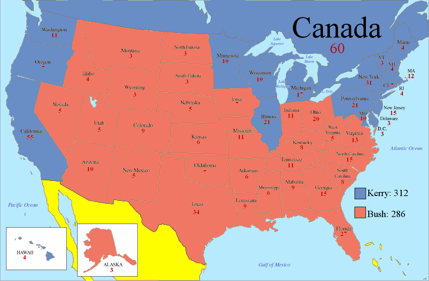
Here’s what would happen in the 2004 presidential election, which President George W. Bush won:

Senator John Kerry wins a pretty clear victory in the electoral vote. He gains 409 electoral votes to Mr. Bush’s 286 and is easily elected president.

What states would Mr. Bush need to flip to win?

In the previous post, where Canada was added to the United States, Mr. Bush would merely have needed to flip one: Wisconsin. Given his 0.4% loss in the state, this would require convincing only 6,000 voters to switch.

Mexico is a lot harder. In order to win, Mr. Bush needs to shift the national vote 4.2% more Republican. This flips six states: Wisconsin, New Hampshire, Pennsylvania, Michigan, Minnesota, and finally Oregon (which he lost by 4.2%). They go in order of the margin of Mr. Bush’s defeat to Mr. Kerry:

But there’s a caveat here: in this scenario the entirety of Mexico is assumed to only have two senators. The fifty states have 435 representatives and 100 senators, making for 535 electoral votes in total (plus Washington D.C.’s three). Mexico, on the other hand, has 158 representatives and two senators, making for only 160 electoral votes. Obviously, Mexico’s influence is strongly diluted.

Mexico itself is organized into 31 states and one federal district. Assume that instead of the entire country voting as one unit, Mexico is divided in the electoral college into these districts. Each Mexican state (and Mexico City) would receive two senators, giving Mexico 222 electoral votes instead of 160.

But that’s not all. There are several states in America – Wyoming, for instance – whose influence is magnified due to their low population. The “Wyomings” of Mexico are Baja California Sur, Colima, and Compeche – which each have less than a million residents. Overall, this would probably add three more electoral votes to Mexico.

This means that Mr. Bush has to flip three more states to win:

New Jersey, Washington, and Delaware go Republican under this scenario. To do this, Mr. Bush would have to shift the national vote 7.59% more Republican (the margin by which he lost Delaware).

One can see that Mexico has a far more powerful effect than Canada; a double-digit Republican landslide has turned into a tie here. That’s what happens when one adds a country of more than one hundred million individuals.

Before Democrats start celebrating however, one should note that this the hypothetical to this point has been in no way realistic. It assumes that the residents of America will not alter their voting habits in response to an extremely fundamental change.

The next post explores some conclusions about what the typical election would look like if the United States became part of Mexico.

–Inoljt

This is the second (more serious) part of two posts exploring the political consequences that would happen if Canada became part of the United States. The previous part can be found here.

A note to all Canadian readers: this post was written for the intent of a good laugh, and some serious political analysis along with it. It is not meant to offend, and sincere apologies are offered if any offense at all is taken.

More below.

How Important Would Canada Be?

The previous post looked at what would have happened in the 2004 presidential election if Canada had been part of the United States:

Democratic candidate John Kerry wins, but barely so. If 6,000 votes had shifted in Wisconsin, here is what would have happened:

Suddenly President George W. Bush is re-elected again.

This example probably overstates the importance of Canada. Canada’s Democratic vote would probably have sent Vice President Al Gore to the White House. But before that, one has to go all the way back to 1876 to find an election when the result would have been changed by Canada voting Democratic. Indeed, before 2000 the last time it matters which way Canada votes comes in 1916.

America’s presidents would mostly have been the same with or without Canada.

Here is another way to look at the picture. In the 2008 presidential election, a total of 131.2 million Americans voted. In the same year Canada held federal elections, in which 13.8 million Canadians voted. If one assumes that the same number of Canadians would vote in an American presidential election, one can make the table below:

If Canada Votes…	Then Barack Obama Gains:
100% Democratic	9.53%
90% Democratic	7.70%
80% Democratic	5.83%
70% Democratic	3.93%
65% Democratic	2.96%
60% Democratic	1.98%
55% Democratic	1.00%

To be fair, these are not bad figures for Democrats. An increase of three percent in one’s popular vote is nothing to sniff at. At the same time, however, it is nothing world-altering.

Let’s take a look at the 2010 midterm elections. 87.8 million Americans voted for a congressional representative, and Republicans won that vote nationally by 6.8%. One can run the same numbers with Canada’s 2008 federal elections to get:

If Canada Votes…	Then Republicans Win By:
100% Democratic	-6.81%
90% Democratic	-4.24%
80% Democratic	-1.60%
70% Democratic	1.12%
65% Democratic	2.51
60% Democratic	3.92%
55% Democratic	5.35%

This indicates that Democrats would have needed around about three-fourths of the Canadian vote to tie in the 2010 popular vote.

Conclusions

A Canadian 51st state of the United States would not change American politics enormously. Ultimately Canada is just not populated enough to fundamentally alter the status quo.

To be sure, the Democratic Party would probably do a bit better initially. Liberal policies would be a bit more popular; conservative policies a bit less so. Canada would help Democrats in the House of Representatives, probably giving them around two dozen extra representatives (although Democratic strength would probably be diluted by the Quebec independence vote). On the presidential level, Democrats would need the Midwest a bit less. They could win with the John Kerry coalition – but barely so.

The beauty of the two-party system, however, is that the Republican Party would eventually adjust. It would move leftwards, much as it did after the New Deal or Democrats moved rightwards after the Reagan years. Eventually, after adopting more liberal policies, the two parties would again approach equilibrium.

Now…it’s a whole different story if Mexico was part of the United States (and not necessarily one that Democrats would like).

–Inoljt

This is the first part of two posts exploring the political consequences that would happen if Canada became part of the United States. The second part can be found here.

A note to all Canadian readers: this post was written for the intent of a good laugh, and some serious political analysis along with it. It is not meant to offend, and sincere apologies are offered if any offense at all is taken.

Now…onto the post.

More below.

Part 1: What If Canada Was Part of the United States?

It is November 2nd, 2004. Election night. Incumbent president George W. Bush is nervously watching election returns, joined by his family. Early exit polls showed him losing massively, but the actual results are far more favorable to him.

As the night goes on, Mr. Bush begins to feel more comfortable. He’s ahead in the key swing states. Florida is going for him far more strongly than anybody expected, and things are also looking good in Ohio. It also looks like Mr. Bush has picked up a couple of states from 2000.

Although opponent Senator John Kerry has yet to concede, the celebration at party headquarters has already started. Drinks are opened. People begin cheering.

Then chief strategist Karl Rove comes in, ashen-faced. He turns to the president. “We’re in big trouble. Canada and California are just about to report, and I don’t think that we have the electoral votes to overcome them.”

Mr. Bush is befuddled. “What? Canada’s part of the United States? I always thought it was a different country.”

Mr. Rove looks puzzled. “No,” he says extremely slowly. “It became part of the United States after the War of 1812.  Are you all right, sir?”

Mr. Bush laughs. “Of course I’m fine. Just wasn’t thinking for a moment. Of course Canada’s part of the United States. Always has been.”

Unfortunately, Mr. Bush’s presidency is not fine. Deep into the night, as the Arctic territory of Yukon finishes voting, Canada reports. Mr. Bush loses badly, gaining only 35% of the vote. Canada’s 50 electoral votes go to Mr. Kerry. Early next morning Mr. Bush telephones his opponent, conceding defeat. Senator John Kerry has just been elected president of the United States.

Canada in the Electoral College

How likely is this scenario?

Well, of course Canada will not probably not become part of the United States anytime soon. Most Canadians are perfectly happy being separate from America. There is little to suggest that this will ever change.

Nevertheless, it is still quite fun to think about the possibilities.

A state’s electoral vote is based off the number of representatives and senators it has in Congress. For instance, California has 53 representatives and 2 senators, making for 55 electoral votes.

According to Canada’s population clock, the nation has an estimated 34,400,000 people (as of March 2010). This is slightly less than California.

The United States Census estimates its population at approximately 308,745,538 individuals. The House of Representatives has 435 individuals, each of whom represents – on average – approximately 709,760 people. If Canada was part of the United States, this would imply Canada adding 48 (rounding down from 48.47) representatives in the House.

This is a simplified version of things; the process of apportionment is quite actually somewhat more complicated than this. But at most Canada would have a couple more or less representatives than this. It would also have two senators, adding two more electoral votes to its 48 representatives.

Canada would thus add around 50 electoral votes in the electoral college:

These votes would almost certainly be Democratic ones. Most people would agree that Canada is a more liberal place than the United States. This is fairly apparent in the policies Canada pursues; it has universal health care and is less skeptical of climate change than the United States. It would not be too unreasonable to suggest, therefore, that Canada would vote for the more liberal party.

Canada’s Importance

Adding another California to the United States would definitely be a good thing for the Democratic Party. Nevertheless, one should not overemphasize Canada’s importance. After all, it’s population is barely one-tenth that of the United States.

Indeed, Mr. Kerry would have barely squeaked to victory with Canada’s electoral votes. In this hypothetical scenario, Mr. Bush would have just needed nine more electoral votes to win.

Here is one such scenario:

Here Mr. Kerry loses Wisconsin – and suddenly George W. Bush is president again.

This is an entirely possible scenario. Mr. Bush lost Wisconsin by 0.4%. A shift of less than 10,000 votes would have given Mr. Bush the state.

While the addition of Canada would shift America leftward, it is easy to overstate the degree of this. The next post will explore this topic more.

–Inoljt

This is part of three posts analyzing the 2010 South Carolina  gubernatorial election, in which Republican Nikki Haley won a  closer-than-expected victory over Democrat Vincent Sheheen. The main  focus of these posts will be to explore whether a racial effect  accounted for Ms. Haley’s unexpected poor performance.

(Note: This is also part of a series of posts analyzing the 2010 midterm elections.)

More below.

The previous post mapped out the relationship between Democratic shifts in 2010 and white registration numbers. Here is the relevant map reposted:

The post ended by noting that “So far this analysis has been relatively light on the statistical side of things.” It included a number of maps, but did not use any raw numbers.

This post aims to draw conclusions based on those numbers.

Let’s begin by translating the picture above into a graph:

This graph maps the relationship between how white a county in South Carolina is, and how much it shifted against non-white Republican candidate Nikki Haley in 2010.

If normally-Republican whites moved against Ms. Haley due to her race, one would expect the dots to be graphed in a roughly 45-degree diagonal line; the whiter a county, the more Democratic it would shift in 2010.

Clearly this is not the case in the graph above. There are a lot of very white counties that shifted strongly against Ms. Haley – but there are also a lot of very white counties that supported her more than they did Senator John McCain.

Indeed, the whitest counties seem to spread out into two groups; one group moves strongly against Ms. Haley, another actually shifts for her. One might speculate that the former group is composed of lower-income, rural whites and the latter is composed of higher-income, metropolitan whites.

To test this theory, the previous post adjusted for income by eliminating all the counties with a median household income greater than the state median (i.e. it got rid of the rich whites). Here is what the result looked like:

There seems to be a correlation here, as the previous post noted.

Here is how the relationship looks on a graph:

The group of white counties which shifted towards Ms. Haley has disappeared. Instead, one sees a much stronger trend: the whiter the county, the more strongly it moved against non-white Republican Governor Nikki Haley.

This only happens once high-income white counties are tossed out of the analysis. High-income Republican whites were very comfortable voting for non-white Republicans; low income Republican whites were less willing.

Interestingly, this pattern is not unique to South Carolina. In Louisiana, Republican Governor Bobby Jindal – a non-white individual of Indian descent – did extremely poorly amongst rural, low-income (Republican) whites while winning landslide support amongst high-income, suburban (Republican) whites. This caused Mr. Jindal to lose in his first attempt to run for governor.

Finally, one can test whether the effect above is statistically significant, or just the result of randomness.

Here is a regression analysis run on the 2010 South Carolina gubernatorial race:

Regression analysis is something I am still not fully comfortable with, so bear this in mind as the analysis continues.

The regression attempted to use two variables – race and income – to predict whether voters would vote more Democratic in 2010. Specifically, it used the percent of white registered voters in a county and said county’s median household income.

The model states that every 10% increase in white registered voters results in a 3.65% greater Democratic shift against Ms. Haley (this is the Coefficient column at the bottom left).

More importantly, whiteness and income were statistically significant when placed together; there was a 0.1% chance that the effect of whiteness was random, and a 0.4% chance that the effect of income was random (this is the P>|t| column at the bottom center).

So the evidence is fairly strong that racially-based voting by low-income whites hurt non-white Republican Ms. Haley in 2010.

There is, however, a caveat. The above regression only explains 20% of the variance between the different degrees of Democratic shifts between different counties (this is the Adj R-Squared line at the top right). This means that 80% of the variance is not explained by race and income.

Racism probably hurt Ms. Haley in 2010, but it was far from the only factor.

–Inoljt

.

.

.

P.S. Here is the relevant data used to built this analysis:

County	% Change   Democratic	% White   Registered	Median   Household Income
Abbeville	21.31%	69.08%	33,995
Aiken	-1.30%	75.02%	43,845
Allendale	1.65%	25.09%	23,942
Anderson	15.75%	83.40%	41,399
Bamberg	-1.54%	37.56%	28,266
Barnwell	0.40%	55.31%	30,549
Beaufort	-8.27%	79.47%	54,085
Berkeley	-1.32%	68.74%	49,609
Calhoun	4.72%	54.90%	39,537
Charleston	-5.41%	69.36%	46,145
Cherokee	14.40%	77.45%	35,807
Chester	4.69%	59.40%	33,640
Chesterfield	15.82%	64.00%	32,267
Clarendon	2.28%	48.66%	29,840
Colleton	1.83%	58.16%	35,935
Darlington	6.87%	56.31%	34,577
Dillon	7.62%	49.11%	28,653
Dorchester	-2.37%	72.07%	52,443
Edgefield	0.86%	62.79%	38,885
Fairfield	4.28%	42.02%	32,694
Florence	6.49%	58.12%	39,919
Georgetown	-2.40%	66.73%	40,573
Greenville	4.41%	78.49%	45,917
Greenwood	12.18%	68.35%	39,586
Hampton	3.50%	42.67%	32,253
Horry	-5.72%	85.98%	41,163
Jasper	-4.05%	47.30%	35,163
Kershaw	33.41%	72.24%	45,268
Lancaster	9.10%	75.12%	40,286
Laurens	10.15%	71.81%	36,910
Lee	7.02%	37.11%	28,041
Lexington	15.99%	84.74%	52,062
Marion	5.55%	41.82%	28,437
Marlboro	9.87%	44.75%	26,799
McCormick	-7.63%	57.41%	35,557
Newberry	13.21%	69.01%	37,263
Oconee	17.25%	91.39%	39,840
Orangeburg	2.19%	34.54%	33,567
Pickens	15.13%	91.76%	40,357
Richland	7.18%	49.90%	45,643
Saluda	15.99%	70.11%	40,819
Spartanburg	7.39%	76.07%	40,278
Sumter	-0.65%	48.08%	37,113
Union	21.54%	67.31%	32,361
Williamsburg	1.43%	31.59%	26,639
York	-5.13%	78.89%	50,644
Total	4.52%	69.66%	42,580

This is the second part of three posts analyzing the 2010 South Carolina  gubernatorial election, in which Republican Nikki Haley won a  closer-than-expected victory over Democrat Vincent Sheheen. The main focus of these posts will be to explore whether a racial effect  accounted for Ms. Haley’s unexpected poor performance.

The previous post can be found here, and the next post can be found here.

(Note: This is also part of a series of posts analyzing the 2010 midterm elections.)

More below.

How to Find a Racial Effect

The purpose of this series of posts is to determine whether or not Ms. Haley’s relatively weak performance was due to a racial effect.

In order to due this, it’s necessary to define what to look for. In this case, it would be normally Republican voters abandoning Ms. Haley due to her race.

Now, South Carolina is a state in which less than 5% of the population is neither white nor black; minorities other than blacks play a negligible role in the state’s politics. It is also a very racially polarized state, like most places in the  Deep South. Blacks vote Democratic; whites vote Republican.

There is one final factor to take into account. When Republican Bobby Jindal ran for governor in 2003 and faced racially-based opposition by (white) Republicans, such opposition was not evenly distributed. The Republicans who abandoned Mr. Jindal tended to be predominantly from rural, relatively lower income areas. This is something that is not especially surprising, although it conforms to some unfortunate stereotypes.

For these reasons, an examination of Republicans who abandoned  Ms. Haley for racial reasons would look specifically at areas with lower-income whites. These areas would be expected to shift more Democratic than the norm.

Democratic Shifts

To begin this post, let’s examine the places where Republicans improved upon their 2008 performance, and the places where Democrats improved upon 2008.

Naturally, given that Ms. Haley did worse than Mr. Sheheen, one would expect Democrats to have relatively more improvement.

This turns out to be the case:

Here one sees a very interesting regional pattern, a pattern that I did not expect when making this map.

The northern parts of South Carolina moved strongly Democratic in 2010. The sole exception is York County, which for whatever reason shifted Republican (there is, strangely enough, very little that differentiates this county with others in the region; nor did either Ms. Haley or Mr. Sheheen represent the county as politicians before 2010).

On the other hand, the coastal regions actually supported Ms. Haley more than they did Senator John McCain.

This is a very interesting regional divide; it is something that is entirely hidden by normal partisan patterns.

Whites

Now, let’s take a look at white registration figures:

This map shows what percent of South Carolina’s registered voters are white. The information is mandated by the Voting Rights Act, given South Carolina’s history of preventing minorities from voting, and can be found at this website. It is also quite useful for the purposes of this analysis. (For fun: compare this map to President Barack Obama’s performance).

In order to make comparisons easier, the same color scale was used in this map as in the previous map. The whiter a county’s voter population, the bluer the county on the map.

If white Republican voters rejected Ms. Haley due to her race, then the whitest counties here would also have the strongest Democratic shift (i.e. the colors in each map would roughly match).

Let’s compare the maps:

There is a bit of a match, but not much. A lot of very white counties shift strongly against Ms. Haley, but a lot of them also shift strongly for her (especially along the coast).

One can reasonably conclude that a lot of white voters – i.e. Republicans – remained loyal to Ms. Haley despite her Indian heritage.

This is not entirely unexpected. Mr. Jindal also retained a large amount of white support, mainly amongst suburban and wealthy whites.

Adjusting For Income

Where Mr. Jindal did especially poorly – and why he lost the 2003 gubernatorial election – was amongst rural, lower income whites in Louisiana.

Let’s therefore shift this analysis by adjusting for income; in other words, by focusing upon lower-income counties in South Carolina.

South Carolina’s median household income was $42,580 as of 2009, according to Census Data (which can be accessed here).

One can therefore adjust for income by restricting the analysis only to those counties in which median household income was below the state median.

This is what happens:

This looks like a far stronger relationship. In the poorer parts of South Carolina, it appears that the whiter the county, the more against Ms. Haley it shifted.

It seems that we have found something here.

So far this analysis has been relatively light on the statistical side of things; it kind of looks like there is a pattern in the map above, but perhaps there isn’t one. How likely is it that this could have occurred by chance?

The next post will answer this question.

–Inoljt

This is the first part of three posts analyzing the 2010 South Carolina gubernatorial election, in which Republican Nikki Haley won a closer-than-expected victory over Democrat Vincent Sheheen. The main focus of these posts will be to explore whether a racial effect accounted for Ms. Haley’s unexpected poor performance.

The next post can be found here.

(Note: This is also part of a series of posts analyzing the 2010 midterm elections.)

More below.

It was the October, 2010 in South Carolina. Nikki Haley, Republican candidate for South Carolina governor, was cruising. She was a conservative candidate – endorsed by none other than Sarah Palin herself – running in a conservative state, in the best Republican year in a generation.

Opinion polls showed the Republican politician leading by double-digits. Even the most pessimistic gave Ms. Haley a high single digit lead.

On election day, however, Ms. Haley won by only 4.5%:

(Note: Edited NYT Image)

What could have accounted for Ms. Haley’s poor performance?

Several factors come to mind. Ms. Haley was not an uncontroversial candidate; her positions were conservative even for South Carolina. The Democratic candidate, Vincent Sheheen, might have been an unnaturally talented campaigner. And there is always the factor of randomness to take into account. There were hundreds of races in November; the polls would inevitably be inaccurate on one or two, and this race just happened to be one of them.

Or perhaps there is another explanation – a particularly ugly one, but one that lurks at the back of everybody’s head. Ms. Haley was an woman of Indian heritage running to govern South Carolina, a state with not exactly the most innocent racial history. Throughout the campaign, Ms. Haley was subject to attacks that implicitly played up the racial angle: she had had affairs with white men (unfortunately for the accusers, this attack doesn’t work as well against women), she wasn’t Christian or was only pretending to be one, and so on.

It is not unimaginable that a sort of Bradley effect took place in South Carolina, that a number of normally steadfast Republicans balked at voting for the first non-white and female governor in history.

This is a serious accusation, and therefore needs serious evidence. The next post will therefore begin an extensive examination of whether Ms. Haley’s race undermined her performance.

–Inoljt

This is a part of a series of posts analyzing the 2010 midterm elections. This post will focus on the Illinois Senate election, in which Republican candidate Mark Kirk pulled out a close Republican victory in a strongly Democratic state.

Illinois’s Senatorial Election

More below.

Senator Mark Kirk’s victory follows the contours of a previous post, titled Previewing Senate Elections: Illinois. This post argued:

So what does Mr. Kirk have to do? Say that  he gets 35% of the vote in Cook County – propelled by inner-ring  suburban strength and minority apathy – and wins a landslide everywhere  else in the state (for instance, a 3:2 margin). This gives him 50.3% of  the vote in the 2008 Illinois electorate. If white Republicans downstate  turn out, and minorities in Chicago do not, Mr. Kirk may get bumped up  to a 2-3% victory.

As it turns out, this is almost exactly what actually happened in the election.

The previous analysis divided Illinois into three sections: Chicago, the suburbs of Chicago, and downstate Illinois. Let’s take a look at what Mr. Kirk did in each part of Illinois.

Chicago

Illinois is generally a Democratic stronghold. Cook County, home to the  city of Chicago, composes more than 40% of the state’s population, and  Democrats always win by a landslide in the county. Republicans have to  stretch themselves to the limit everywhere else in the state – winning  even the areas that normally vote Democratic – to get close.

But Republicans also must dampen Democratic margins in Cook County. This happens if Republicans can do well in the parts of Cook County outside Chicago, which are whiter and more conservative. In the city of Chicago itself, most voters are so Democratic that they will prefer not voting to casting the ballot for a Republican. There, low turn-out is more important for Republicans than actually winning over voters.

In 2010, Democratic candidate Alexi Giannoulias won 64.3% of the vote in Cook County.

At first glance, this sounds quite good. Winning 64.3% of the vote is nothing to sniff at. No president has ever won that much of the popular vote in history.

But Senator John Kerry won 70.2% of the vote in Cook County. And President Barack Obama took 76.2% of the vote. In modern Illinois politics, a Democratic candidate who takes only 64.3% of the vote in Cook County is in deep trouble.

Chicago’s Suburbs

“Previewing Senate Elections, Illinois” stated that:

The true test of Mark Kirk’s candidacy will come in the Chicago suburbs…

He will not just have to win the suburbs, but  turn the clock back two decades – back to the glory years in which  Republicans won around 70% of the vote in DuPage County. (Mr. Kirk will  probably not have to do that well, given rising Republican strength  downstate.)

Is this doable? Given that Republicans seem  to be winning suburbs everywhere this year, it is certainly possible.  Mr. Kirk, moreover, has spent a decade representing a Chicago suburb  congressional district; this is why Republicans have nominated him.

As it turned out, Mr. Kirk passed the test with flying colors. His moderate image and suburban origin led to double-digit victories in every one of the collar counties surrounding Cook County.

In the past, Republicans have won Illinois through massive support in the Chicago’s suburbs to offset the Democratic advantage in Chicago itself. Mr. Kirk was able to somewhat replicate this model in 2010:

This strength did not extend to all Republicans. Republican candidate Bill Brady, for instance, still won the Chicago suburbs. But his margins were just the slightest bit off – a high single-digit rather than double-digit victory here; a 15-point rather than 20-point margin there – and ultimately this led to Mr. Brady’s defeat.

Downstate Illinois

Imagine that the year is 1990, and Republican Mark Kirk pulls the exact same numbers in the Chicago metropolis.

Most analysts in that year would say that Mr. Kirk is on his way to a sure loss – after all, Democrats are quite competitive in downstate Illinois, and Mr. Kirk just hasn’t squeezed enough juice from the collar counties.

Today, however, downstate Illinois has trended firmly Republican. Without this trend Mr. Kirk would not have won.

Here is an illustration of Illinois in the 1992 presidential election:

President Bill Clinton is doing quite well, winning almost every single county downstate – many by double-digits. Compare this to President Barack Obama’s performance:

Mr. Obama is actually doing much better in Illinois than Mr. Clinton, and yet he loses a number of the downstate counties Mr. Clinton won.

This illustrates the shift in downstate Illinois to the Republican side, and in 2010 Mr. Kirk took full advantage of that trend to win re-election.

Conclusions

The post “Previewing Senate Elections: Illinois” concluded by mapping, somewhat light-heartedly, a hypothetical Republican victory:

Mr. Kirk’s victory ended up looking extremely similar:

All in all, it is always exciting to see a Republican victory in a Democratic  stronghold, or a Democratic victory in a Republican stronghold. Mr.  Kirk’s victory is the first time a Republican has won Illinois in quite a  while. It constitutes one of the Republican Party’s greatest triumphs  in the 2010 midterm elections.

–Inoljt

Asians are one of the most ignored constituencies in American politics. When most politicians think about the Asian vote, they don’t.

Yet the Asian-American population is increasing, both in absolute terms and relative ones. By 2050, the Census estimates that Asians will compose 7.8% of the American population. Although their voting rates will still fall far short of this, the population is becoming more influential. Predicting their future voting path therefore has some utility.

In previous posts, this blogger has argued that the Latino vote will likely trend Republican, as Latinos follow the path of previous immigrants and become more assimilated.

Will the same happen for Asian-Americans?

More below.

Probably not:

As the graph above shows, the Asian vote has steadily moved Democratic, in quite a significant manner. In 1992 Republican President George H.W. Bush won 55% of the Asian vote while losing the popular vote. 12 years later, his son won only 41% of Asians, despite winning the popular vote.

The trend also does not look bright for the Republican Party. Asian-Americans who have been born in the United States are, if anything, more Democratic than those who immigrated into the country (to be fair, the latter group dominates the Asian population and will continue to do so unless immigration is drastically curtailed).

Take, for instance, the Vietnamese-American population – strong supporters of the Republican Party. The Asian American Legal Defense and Education Fund, after conducting an extensive exit poll of Asians (perhaps the only detailed exit poll of the group in the country), found that:

Vietnamese American voters gave McCain the strongest support of all Asian ethnic groups at 67%. However, further analysis of Vietnamese American voters revealed 69% of those born in the U.S. and 60% of those 18-29 years old voted for Obama. Among Vietnamese American respondents, 15% were born in the U.S. and 25% were between the ages of 18 and 29.

The analysis goes on to conclude that:

AALDEF’s exit poll data shows that younger, U.S.-born, more recently naturalized, and English proficient Asian American citizens voted for Barack Obama for President by wide margins. Older, foreign-born citizens with limited English proficiency and who had been naturalized more than ten years ago voted in greater proportions for McCain.

There are several explanations for why this is happening. One quite plausible argument is that immigration has shifted the Asian-American population from Orange County anti-communists to Silicon Valley liberals.

Another revealing insight can be gained by comparing Asians to another very Democratic group: Jews. In many ways the two have a startling amount in common. Both groups are highly educated; both are primarily located in urban metropolitan areas; both have achieved substantial success in American society; and both have encountered quite similar types of discrimination. Even the stereotypes are similar.

Given these similarities, it is very conceivable that Asians could end up voting like Jews – one of the most liberal-minded groups in the nation.

–Inoljt, http://mypolitikal.com/

This is the second part of two posts analyzing in more detail the 1928 presidential election.

The Great Realignment

The previous post noted that:

In 1928 the Democratic Party nominated Governor Al Smith of New York. Mr. Smith was nominated as a Catholic Irish-American New Yorker  who directly represented Democratic-voting white ethnics. Mr. Smith’s  Catholicism, however, constituted an affront to Democratic-voting white  Southerners, who at the time were the most important part of the party’s  base.

The 1928 presidential election thus saw a mass movement of white  Southerners away from the Democrats, corresponding with a mass movement  of white ethnics towards the Democrats. This was the beginning of the  great realignment of the South to the Republican Party and the Northeast  to the Democratic Party.

This change can be illustrated with a map detailing the state-by-state shift from the 1924 presidential election to the 1928 presidential election:

There are a number of things that stand out with this map.

More below.

The first, as has been previously noted, is the degree to which the shift replicates the current electoral map.

This is not all, however. Two other things are very, very out-of-whack here. To get a hint at what these are, it is useful to compare the 1924 to 1928 state-by-state voting shift to that of different elections.

One example is the change from 2004 to 2008.

In 2008 President Barack Obama improved by 9.7% from the performance of the previous Democratic candidate, Senator John Kerry. In 1928 Governor Al Smith improved by 7.8% from the performance of Democratic candidate John Davis. The shift from 1924 to 1928 is therefore roughly comparable to the shift from 2004 to 2008.

Here is a map of that shift:

Although both Democratic candidates improved by roughly the same percentage from the previous election, where and how they improved look completely different.

In 2008, Mr. Obama generally improved everywhere. In only five states does he do worse than Mr. Kerry. This is the famous Appalachian corridor with which Mr. Obama was so weak.

Moreover, the degree of movement is generally modest. Only two states – Hawaii and Indiana – have more than a 20-point shift from how they voted in 2004. No state shifts more than 40 points (although Hawaii certainly comes close, going from a 8.7% Democratic margin to a 45.3% Democratic margin).

These two patterns: uniform and moderate movement (i.e. when a candidate does better in the popular vote, said candidate does better in almost every state, and states generally do not have wild swings from how they voted from the previous election) are not just confined to 2008. Here is the shift from 2000 to 2004, when President George W. Bush improved by 2.9% from his performance four years earlier:

One again we see that the national shift right brought most of the states with them, and that only three states shifted more than 10% from 2000.

Let’s take another look at 1928 to finish:

Here neither pattern is present. In 1928, the country moved 7.8% more Democratic from 1924. Despite this, Democratic candidate Al Smith did worse in 23 out of 48 states. Three states – Florida, Georgia, and Texas – voted more than 40% more Republican than they did in the previous election. In Texas, Republicans went from 19.8% of the vote in 1924 to 51.8% of the vote in 1928. Fifteen states voted more than 10% more Republican than they did in 1924.

In comparison, in 2008 only one state – Arkansas – voted more than 10% more Republican than it did in 2004 (and it did so by the barest of margins: 10.1%). This was despite Mr. Obama’s improvement from 2004 being roughly equivalent to Mr. Smith’s improvement from 1924.

A lot of interest has gone into Mr. Obama’s weakness in Appalachia. But Mr. Smith’s Southern problem in 1928 (i.e. the fact that he was a Catholic) makes Mr. Obama’s Appalachian problem look puny.

If Mr. Smith improved by 7.8% from the performance of his Democratic predecessor with so much weakness in the South, the shift in the states that voted more Democratic must have been huge. And indeed, the New Yorker gained more than 20-point shifts in nine states. In Massachusetts, Democrats went from 24.9% of the vote in 1924 to 50.2% in 1928.

All in all, the 1928 presidential election was the scene of some enormous movement on a state-by-state basis. In 2008 only two states shifted more than 20 points from 2004, as Mr. Obama did 9.7% better than Mr. Kerry. In 1928, on the other hand, sixteen states shifted more than 20 points from 1928, as Mr. Smith did 7.8% better than the previous Democratic candidate.

This is what a realigning election looks like – extreme movement on from one state to the next, enormous differences by region, and a powerful correlation between which states shift Democratic and which states are voting Democratic almost a century later.

P.S. For those interested, here is a table of the state-by-state voting shift from the 1924 presidential election to the 1928 presidential election:

State	1928 Republican   Margin	1924 Republican   Margin	Change
Alabama	-2.84%	–40.80%	37.96%
Arizona	15.34%	5.79%	9.55%
Arkansas	-20.96%	-31.93%	10.97%
California	30.50%	48.97%	-18.47%
Colorado	30.78%	35.04%	-4.26%
Connecticut	8.06%	34.01%	-25.95%
Delaware	30.42%	20.90%	9.52%
Florida	16.72%	-28.82%	45.54%
Georgia	-13.19%	-55.77%	42.58%
Idaho	29.30%	30.76%	-1.46%
Illinois	14.65%	35.48%	-20.83%
Indiana	20.09%	16.56%	3.53%
Iowa	24.20%	38.39%	-14.19%
Kansas	44.96%	37.94%	7.02%
Kentucky	18.82%	2.95%	15.87%
Louisiana	-52.58%	-56.21%	3.63%
Maine	37.66%	50.20%	-12.54%
Maryland	14.74%	4.00%	10.74%
Massachusetts	-1.09%	37.40%	-38.49%
Michigan	41.44%	62.24%	-20.80%
Minnesota	16.94%	44.38%	-27.44%
Mississippi	-64.20%	-81.79%	17.59%
Missouri	11.43%	5.79%	5.64%
Montana	17.89%	23.12%	-5.23%
Nebraska	27.01%	17.51%	9.50%
Nevada	13.07%	19.81%	-6.74%
New Hampshire	17.63%	25.11%	-7.48%
New Jersey	19.97%	34.76%	-14.79%
New Mexico	18.16%	5.50%	12.66%
New York	2.35%	26.63%	-24.28%
North Carolina	9.87%	-19.16%	29.03%
North Dakota	10.34%	40.72%	-30.38%
Ohio	30.43%	34.63%	-4.20%
Oklahoma	28.28%	-5.59%	33.87%
Oregon	30.04%	26.83%	3.21%
Pennsylvania	31.35%	46.26%	-14.91%
Rhode Island	-0.61%	23.17%	-23.78%
South Carolina	-82.85%	-94.35%	11.50%
South Dakota	20.98%	36.34%	-15.36%
Tennessee	7.72%	-9.21%	16.93%
Texas	3.67%	-53.92%	57.59%
Utah	7.72%	19.32%	-11.60%
Vermont	34.00%	62.55%	-28.55%
Virginia	8.01%	-29.69%	37.70%
Washington	35.75%	42.08%	-6.33%
West Virginia	17.39%	5.38%	12.01%
Wisconsin	9.24%	28.96%	-19.72%
Wyoming	28.31%	36.28%	-7.97%
Total	25.22%	17.42%	-7.80%

–Inoljt

This is the first part of two posts analyzing in detail the 1928 presidential election.

The second post can be found here.

The Context

In a previous post, part of a series analyzing the Democratic Party during the 1920s, I spoke of how the 1928 presidential election constituted a realigning election.

The 1928 presidential election marked the beginning of a great shift in American politics. It was when the Democratic Party started changing from a minority and fundamentally conservative organization into the  party that would nominate Senator Barack Obama for president.

In 1928, the Democratic Party nominated Governor Al Smith of New York. Mr. Smith was nominated as a Catholic Irish-American New Yorker who directly represented Democratic-voting white ethnics. Mr. Smith’s Catholicism, however, constituted an affront to Democratic-voting white Southerners, who at the time were the most important part of the party’s base.

The 1928 presidential election thus saw a mass movement of white Southerners away from the Democrats, corresponding with a mass movement of white ethnics towards the Democrats. This was the beginning of the great realignment of the South to the Republican Party and the Northeast to the Democratic Party.

Several maps illustrate this point succinctly. Here is the 1924 presidential election:

Here is the 1928 presidential election:

As one can tell, there is quite a bit of change from the one presidential election to the next. Democratic strength in the Solid South weakens considerably, while the Republican Midwest and Northeast become much less red.

However, it is somewhat difficult to go further into detail just by comparing the two maps. One can sense that a lot is changing, and that certain regions of the country are moving in diametrically opposed directions. But it is all rather vague.

I therefore decided, out of curiosity, to create an actual map of the shift from 1924 to 1928. Here it is:

This is quite the interesting map. One can see the outlines of the current Democratic electoral map here. In some cases the correlation is quite tight. For instance, Indiana is the only state in the Midwest to vote more Republican in 1928 – and what do you know, today Indiana votes the most Republican out of all the states in that region.

In general the relationship is very strong in the eastern half of the country. The only “wrong” states are today’s Democratic strongholds of Maryland and Delaware. Also, the degree of shift does not perfectly correlate to Republican strength in some of the Southern states. But these are small details; in the East, states that moved Democratic in 1928 vote Democratic today, while states that moved Republican in 1928 vote Republican today.

West of Minnesota, however, the relationship breaks down. In more than a third of the states in the West, the way they shifted in 1928 is opposite of how they vote today. The most obvious outlier is Utah, today a rock-solid Republican stronghold that moved sharply Democratic in 1928.

There are two other very interesting and strange things that are happening in this map. They will be the subject of the next post.

–Inoljt