PVI – Swing State Project

The Worst Republican Senate Candidates of 2010, Part 1

This is the first part of two posts analyzing patterns in the 2010 Senate midterm elections. The second part can be found here.

The 2010 congressional midterm elections constituted, by and large, a victory for the Republican Party. In the Senate Republicans gained six seats. While this was somewhat below expectations, it was much better than Republican hopes just after 2008 – when many expected the party to actually lose seats.

The Senate results provide some interesting fodder for analysis. The table below indicates which Republicans Senate candidates did the worst in 2008. It does so by taking the Republican margin of victory or defeat in a given state and subtracting this by the Cook PVI of the state (the Cook PVI is how a state would be expected to vote in a presidential election in the event of an exact tie nationwide). Given that Republicans won the nationwide vote this year, the average Republican candidate would be expected to do better than the state’s PVI. A bad Republican candidate would actually do worse than the state’s PVI.

Let’s take a look at this table below the flip.

State	Republican Margin	Cook PVI	Republican Overperformance
South Dakota	100.00%	8.9%	91.10%
North Dakota	53.91%	10.4%	43.51%
Kansas	43.72%	11.5%	32.22%
Iowa	31.05%	-1.0%	32.05%
Idaho	46.25%	17.4%	28.85%
Oklahoma	44.50%	16.9%	27.60%
Florida	28.69%	1.8%	26.89%
South Carolina	33.83%	7.8%	26.03%
New Hampshire	23.22%	-1.6%	24.82%
Arizona	24.14%	6.1%	18.04%
Alabama	30.47%	13.2%	17.27%
Ohio	17.44%	0.7%	16.74%
Georgia	19.31%	6.8%	12.51%
Arkansas	20.96%	8.8%	12.16%
Missouri	13.60%	3.1%	10.50%
Illinois	1.60%	-7.7%	9.30%
Louisiana	18.88%	9.7%	9.18%
Utah	28.79%	20.2%	8.59%
Indiana	14.58%	6.2%	8.38%
North Carolina	11.77%	4.3%	7.47%
Wisconsin	4.84%	-2.4%	7.24%
Pennsylvania	2.02%	-2.0%	4.02%
Kentucky	11.47%	10.4%	1.07%
Washington	-4.73%	-5.0%	0.27%
Alaska	11.94%	13.4%	-1.46%
Colorado	-1.63%	0.2%	-1.83%
California	-10.01%	-7.4%	-2.61%
Nevada	-5.74%	-1.3%	-4.44%
Connecticut	-11.94%	-7.1%	-4.84%
Delaware	-16.58%	-7.0%	-9.58%
Oregon	-17.98%	-4.0%	-13.98%
New York (S)	-27.84%	-10.2%	-17.64%
Maryland	-26.44%	-8.5%	-17.94%
West Virginia	-10.07%	7.9%	-17.97%
Vermont	-33.41%	-13.4%	-20.01%
New York	-34.10%	-10.2%	-23.90%
Hawaii	-53.24%	-12.5%	-40.74%
Total/Average	5.54%	2.3%	8.08%

(Note: The data in Alaska and Florida refer to the official candidates nominated by the parties, not the independent candidates – Senator Lisa Murkowski and Governor Charlie Crist – who ran in the respective states).

This table reveals some fascinating trends. There is a very clear pattern: the worst Republican candidates ran in the bluest states – and the bluer the state, the more the Republican underperformed. This does not just mean that these Republicans lost, but that they lost by more than the average Republican was supposed to in the state. Republican candidates did worse than the state’s PVI in thirteen states; nine of these states had a Democratic PVI.

There seems to be a PVI tipping point at which Republicans start underperforming: when a state is more than 5% Democratic than the nation (PVI D+5). Only one Republican in the nine states that fit this category overperformed the state PVI (Senator Mark Kirk of Illinois ).

Something is puzzling about this pattern. It is true that states like Connecticut or Maryland will probably vote Democratic even in Republican victories. The Cook PVI predicts that Democrats will win by X% in the event of a national tie in the popular vote. One would thus have expected Republican candidates to do better than this in 2010, given that 2010 was the strongest Republican performance in a generation.

Yet this did not happen. In a lot of blue states Democrats actually did better than the Cook PVI would project them to do – that is, said blue states behaved like the Democrats had actually won the popular vote, which they certainly did not in 2010. The bluer the state, the stronger this pattern.

There are a couple of reasons why this might be. The first thing that comes to mind is the money and recruiting game. The Republican Party, reasonably enough, does not expect its candidates to win in places like New York and Maryland . So it puts less effort into Republican candidates in those states. They get less money – and therefore less advertising, less ground game, and so on. Nobody had any idea who the Republican candidate in Vermont was, for instance. That probably contributes to Republican underperformance in deep-blue states.

The second factor might be a flaw in the model the table uses. Democratic and Republican strongholds, for whatever reason, behave differently from “uniform swing” models. In almost all the counties President Barack Obama won, for instance, he improved upon President Bill Clinton 1992 and 1996 performance – despite the fact that Mr. Clinton won by similar margins in the popular vote. This holds true from San Francisco to rural Mississippi . In the 2010 Massachusetts special Senate election, the most Democratic areas of Massachusetts swung least towards Republican Senator Scott Brown. The fact that the worst Republican candidates ran in the bluest states fits the pattern.

The table presents another startling pattern, which will be discussed in the next post: there are surprisingly few Republicans who did worse than they were supposed to in red states.

–Inoljt

Learning from 1994 (Part II)

This week we’re taking an in-depth, multi-part look at the 1994 election, as a means of divining what the 2010 election may hold for us in the House. To do so, we’re looking at some of the myths that seem to have taken hold regarding 1994; yesterday, for instance, we addressed the idea that 1994 was full of unpredictable, arbitrary wipeouts — which it wasn’t (our House Vulnerability Index did a spot-on job of predicting likelihood of losing compared with other Democrats).

Today, we’re looking at a couple more myths. They’re all interrelated — open seats and freshman status weigh heavily on the House Vulnerability Index — but it lets us slice and dice the data some new ways:

Myth 2) The losses in the 1994 election were disproportionately in the South, as historically Democratic districts that had started going Republican at the presidential level finally flipped downballot too.

No, not true. There’s plenty of reason to think this was the case (as I did until I started doing this research), as the 1992 round of redistricting rejiggered a number of districts in a way that was potentially harmful to moderate white Democrats elected by a coalition of African-Americans and working-class whites. With the creation of odd-shaped VRA-districts in a number of states, starting in 1992, moderate Democrats found themselves with the choice of either primaries against African-Americans in VRA districts, or against Republicans in much more conservative suburban/rural districts.

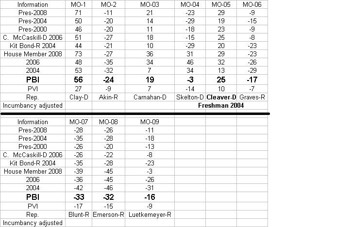
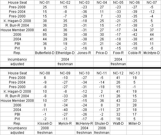
However, it turns out most of the impact from this occurred immediately in 1992, not 1994. For instance, the two Birmingham-area districts, which supported moderate Dems Claude Harris and Ben Erdreich, got turned into the mostly-white 6th and mostly-black 7th, which thus in 1992 turned into liberal Dem Earl Hilliard and conservative GOPer Spencer Bachus. Similarly, in 1992, long-time Democratic Rep. Walter Jones Sr. retired when he found himself in a now black-majority NC-01; his son, Walter Jones Jr., lost the Dem primary to Eva Clayton. In fact, this gave rise to perhaps the only Dem loss in 1994 that seems directly related to the VRA gerrymander: Rep. Martin Lancaster survived the 1992 election reasonably well despite having lost many of NC-03’s African-American voters to next-door NC-01, but in 1994 faced off against the younger Jones, now a Republican (and whose dad had represented many of NC-03’s voters prior to the redistricting), and lost.

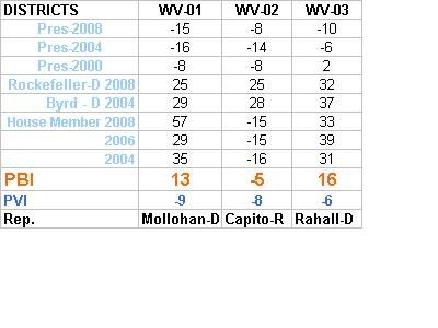
It’s possible that Stephen Neal in NC-05, who got a nastier district in 1992 after having the black parts of Winston-Salem moved into the newly-formed NC-12 and then won by only 7% in 1992, may have felt compelled to hit the exits in 1994 primarily because he didn’t relish the task of trying to hold the district. At R+4 at the time, though, that wasn’t a particularly bad district. Norm Sisisky’s VA-04 also seems to have gotten worse post-1992 because of the gerrymandering of VA-03, but he still survived 1994 unscathed and held that district until his 2001 death. (If you can think of any other examples, please discuss in the comments. For instance, the creation of GA-11 or FL-03 may have had some consequences I’m not thinking of.)

The South (as defined by the US Census with one exception — I’m treating Maryland and Delaware as Northeast) did lose more Democratic seats than any other region of the country, that much is true. But that’s mostly because there were more Democratic seats in the South than any other region of the country; in terms of the overall win/loss percentage, the Democrats actually fared slightly better in the South than in the Midwest or West. In addition, much of what happened in the South was because of open seats; there were certainly more open seats in the South, while the South’s freshmen and veterans tended to fare better than those in the Midwest and West. There may be something of a chicken and egg effect here — old-timer Reps. in the South may have sensed trouble a-brewin’ and gotten out of the way, meaning that the inevitable losses took the form of open seats instead of defeated veterans — but, as we saw yesterday, open seats are the hardest to defend and the mass retirements (15 in the South) seemed to compound the disaster.

The one region where the Democrats performed notably better than the norm was the Northeast (their casualty rate in defensive races was only 11%, compared with 22% overall). That’s largely because there are so many safely-blue districts in the major cities of the Northeast; there were fewer suburban or rural seats there, which were the types that the GOP picked up in 1994. (The Dems faring comparatively well in 1994 in the Northeast helped pave the wave for their near-total dominance there now, as they gradually picked up suburban districts that leaned blue at the presidential level over the following decade.)

—	South	Mid- west	West	North- east	Nationwide
Seats Defended	86	61	55	54	256
All Seats Won	67	45	40	48	200
All Seats Lost	19	16	15	6	56
Casualty Rate	22%	26%	27%	11%	22%
All Open Seats	15	8	4	4	31
Open Seats Lost	11	6	3	2	22
Open Seat Casualty Rate	73%	75%	75%	50%	71%
All Freshmen	22	14	17	13	66
Freshmen Lost	3	4	7	2	16
Freshmen Casualty Rate	13%	29%	41%	15%	24%
All Veterans	49	39	34	37	159
Veterans Lost	5	6	5	2	18
Veteran Casualty Rate	10%	15%	15%	5%	11%

This table also brings us to another myth which we’ll talk about today:

Myth 3) Veterans fell victim to the slaughter just as much as newcomers.

No, not at all. (This myth — which may have arisen just because of the sheer shock of losing Foley and Rostenkowski — we sort of discussed yesterday, in the context of how the losses that were suffered in 1994 were largely predictable. That’s because the House Vulnerability Index that I’ve developed places the highest level of vulnerability on open seats, and then tends to rate frosh as next-most-vulnerable, generally because they usually win their initial election by narrower margins than do veterans. But we’ll talk about it some more today.)

As you can see, the safest place to be in 1994 was among the ranks of veterans (and you’d be extra-safe as a veteran in the Northeast). The GOP picked up the large majority of open seats, and cut a decent-sized swath through the freshmen, but 89% of the veterans lived to fight again. In fact, as you’ll notice from the lists above, the numbers of the freshmen who lost in actually competitive seats (based on Cook Partisan Voting Index) nearly rivals the rate at which open seats fell, if you factor in the large number of freshmen in newly-created 1992 VRA seats that weren’t going to go Republican under any circumstances. Compare the survival rate among freshmen in the South (where most were in new VRA seats) with the survival rate among freshmen in the West (where there was little creation of VRA seats, compounded by the Dems’ particularly egregious — and, to me, rather inexplicable — collapse in Washington state).

If you look at the list of winners and losers in each region in the lists that are over the fold, you can see the point in the PVIs where you shift from D+s to R+s as being the point where open seats and freshmen started falling. In the interest of space, I didn’t list all veterans who survived, but, by contrast, there were many who did so even while in seriously GOP-leaning turf. Was that because they hedged their bets by voting against big-ticket Democratic agenda items like the Clinton budget and the assault weapon ban, which were presumably unpopular in their conservative districts? Well, that’s something we’ll talk about in the coming days.

Here’s the list of who goes where. Open seats, for our purposes, includes races where the incumbent was knocked off in a primary. (And I’m not listing veterans who won, in the interest of space.)

South open seats won: TX-18 (D+22, ex-Washington), TX-10 (D+8, ex-Pickle), KY-03 (D+3, ex-Mazzoli), TX-25 (D+3, ex-Andrews)

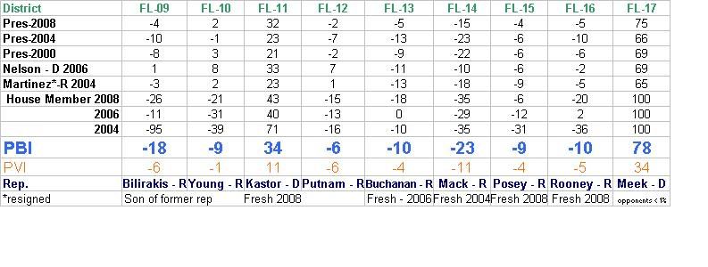
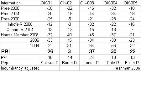
South open seats lost: OK-02 (D+3, ex-Synar), TN-04 (R+2, ex-Cooper), NC-05 (R+4, ex-Neal), TN-03 (R+5, ex-Lloyd), OK-04 (R+7, ex-McCurdy), NC-02 (R+7, ex-Valentine), MS-01 (R+7, ex-Whitten), GA-08 (R+8, ex-Rowland), SC-03 (R+13, ex-Derrick), FL-15 (R+14, ex-Bacchus), FL-01 (R+20, ex-Hutto)

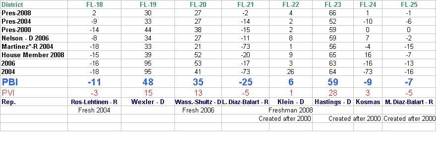
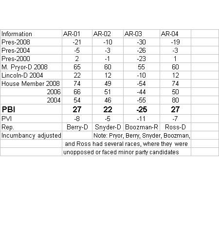
South freshmen won: FL-17 (D+25, Meek), AL-07 (D+21, Hilliard), LA-04 (D+19, Fields), TX-30 (D+19, Johnson), NC-12 (D+18, Watt), VA-03 (D+18, Scott), GA-11 (D+17, McKinney), FL-23 (D+16, Hastings), NC-01 (D+15, Clayton), SC-06 (D+14, Clyburn), GA-02 (D+12, Bishop), TX-28 (D+11, Tejeda), TX-29 (D+11, Green), FL-03 (D+10, Brown), MS-02 (D+9, Thompson), AR-01 (D+7, Lambert), FL-20 (D+3, Deutsch), FL-05 (R+1, Thurman), GA-09 (R+14, Deal)

South freshmen lost: KY-01 (D+0, Barlow), VA-11 (R+5, Byrne), GA-10 (R+10, Johnson)

South veterans lost: TX-09 (D+5, Brooks), NC-04 (D+1, Price), TX-13 (R+5, Sarpalius), NC-03 (R+8, Lancaster), GA-07 (R+11, Darden)

Midwest open seats won: MO-05 (D+13, ex-Wheat), MI-13 (D+4, ex-Ford)

Midwest open seats lost: OH-18 (D+2, ex-Applegate), MN-01 (D+1, ex-Penny), IL-11 (R+1, ex-Sangmeister), MI-08 (R+1, ex-Carr), KS-02 (R+2, ex-Slattery), IN-02 (R+8, ex-Sharp)

Midwest freshmen won: IL-01 (D+34, Rush), IL-02 (D+32, Reynolds), IL-04 (D+19, Gutierrez), WI-05 (D+13, Barrett), MI-05 (D+5, Barcia), MO-06 (D+3, Danner), MI-01 (D+0, Stupak), MN-02 (R+0, Minge), OH-13 (R+1, Brown), ND-AL (R+7, Pomeroy)

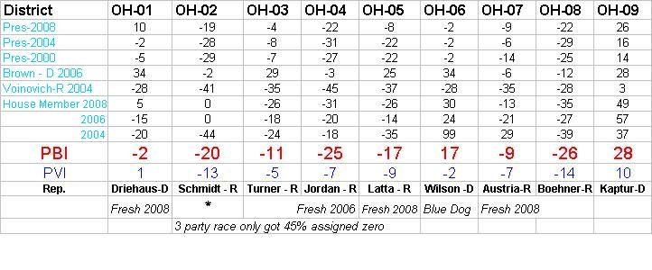
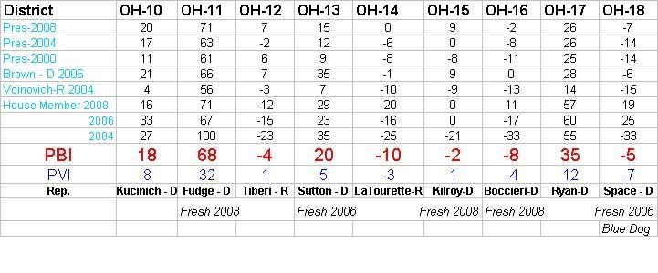
Midwest freshmen lost: WI-01 (D+3, Barca), OH-19 (R+0, Fingerhut), OH-01 (R+2, Mann), OH-06 (R+4, Strickland)

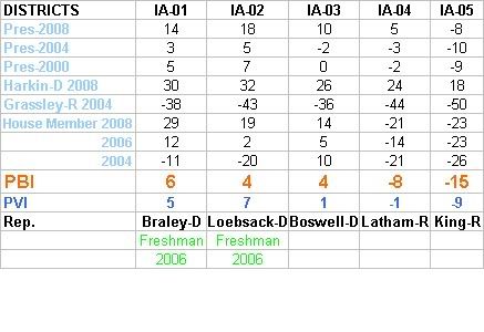
Midwest veterans lost: IL-05 (D+5, Rostenkowski), IA-04 (D+4, Smith), IN-08 (R+2, McCloskey), KS-04 (R+6, Glickman), NE-02 (R+8, Hoagland), IN-04 (R+13, Long)

West open seats won: CA-16 (D+12, ex-Edwards)

West open seats lost: OR-05 (D+2, ex-Kopetski), WA-02 (D+2, ex-Swift), AZ-01 (R+9, ex-Coppersmith)

West freshmen won: CA-37 (D+29, Tucker), CA-30 (D+18, Becerra), CA-33 (D+18, Roybal-Allard), CA-06 (D+15, Woolsey), CA-14 (D+11, Eshoo), CA-17 (D+11, Farr), AZ-02 (D+11, Pastor), CA-50 (D+7, Filner), OR-01 (D+4, Furse), CA-36 (R+3, Harman)

West freshmen lost: CA-01 (D+7, Hamburg), WA-09 (D+3, Kreidler), WA-01 (D+2, Cantwell), CA-49 (D+1, Schenk), AZ-06 (R+4, English), WA-04 (R+7, Inslee), UT-02 (R+8, Shepherd)

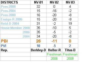
West veterans lost: WA-03 (D+4, Unsoeld), NV-01 (D+1, Bilbray), WA-05 (D+1, Foley), CA-19 (R+4, Lehman), ID-01 (R+9, LaRocco)

Northeast open seats won: PA-02 (D+26, ex-Blackwell), PA-20 (D+11, ex-Murphy)

Northeast open seats lost: ME-01 (R+0, ex-Andrews), NJ-02 (R+4, ex-Hughes)

Northeast freshmen won: NY-08 (D+28, Nadler), MD-04 (D+24, Wynn), NY-12 (D+22, Velazquez), NY-14 (D+20, Maloney), MA-01 (D+10, Olver), PA-04 (D+10, Klink), NJ-13 (D+7, Menendez), MA-05 (D+2, Meehan), NY-26 (D+2, Hinchey), PA-15 (R+1, McHale), PA-06 (R+7, Holden)

Northeast freshmen lost: NJ-08 (R+1, Klein), PA-13 (R+4, Margolies-Mezvinsky)

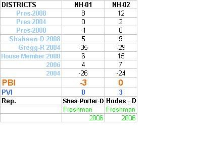
Northeast veterans lost: NH-02 (R+5, Swett), NY-01 (R+6, Hochbrueckner)

Learning from 1994 (Part I)

The ghost of 1994 has kept hanging over the House Democrats’ heads almost this entire Congress. That’s more the product of conventional wisdom feeding upon itself and turning into a self-fulfilling prophecy than anything else, but there are legitimate warning signs on the road ahead: not just the natural pendulum-swinging that occurs during almost every midterm against the party that controls all levels of power, but also clues like the Republicans moving into the lead in many generic congressional ballots and polls showing Republicans competitive in individual House races (although many of those polls are either internals or from dubious pollsters).

On the other hand, there are plenty of reasons to expect that, while the Democrats may lose seats, there won’t be a 1994-level wipeout. There aren’t as many retirements as in 1994 (where the Dems had 28 open seats), and certainly not as many retirements in unpleasantly red seats (17 of those 1994 retirements were in GOP-leaning seats according to the Cook Political Report’s Partisan Voting Index – compared with only 8 facing us in 2010). There are still lots of polls, of the non-Rasmussen variety, giving the Dems an edge in the generic ballot. The DCCC has a sizable financial advantage, and maybe most importantly, the DCCC and its individual members appear acutely aware of the potential danger, unlike in ’94, when they seemed to blithely sail into disaster.

This week we’re going to be doing a multi-part series looking at the House in 1994, trying to draw some parallels and applying those lessons to today. To make this investigation as accessible as possible, we’re going to frame it in terms of a number of myths about 1994, and see how much reality there is to them. For instance, were the members who lost done in by their “yes” votes on tough bills? And was the impact of the post-1992, post-Voting Rights Act redistricting a killer for moderate southern Dems suddenly cast into more difficult districts? Those are problems we’ll look at in the next few days. For today, we’ll start with:

Myth #1: Losses in 1994 were full of surprises: the old and the new, the vulnerable and the safe were swept away together by the tide.

No, not especially true. According to standard diagnostic tools (such as Cook PVI or the 1992 victory margins of individual House members), the vulnerable seats were lost; the not-so-vulnerable seats were retained. The House Vulnerability Index that I’ve applied in several posts to today’s electoral cycle, in fact, does a pretty remarkable job of predicting who would have lost in 1994. If you aren’t familiar with it, it simply combines PVI and previous victory margin into one handy value that rates a particular member’s vulnerability relative to other members of the same party. (For open seats, the HVI uses a victory margin of zero.) It doesn’t predict how likely a person is to lose – that depends heavily on the nature of the year – but it does predict likelihood of losing relative to other members of the party. (Cook hasn’t officially released PVIs for this era as far as I know, but I calculated them based on the 1988 and 1992 presidential election data for each district, according to post-1992 district lines.)

As it turns out, the HVI shows that, of the 25 most vulnerable seats in 1994, 23 were lost to the Republicans. Of seats 26 through 50, another 13 were lost. And of pre-1994 Democratic House members outside the top 100 in terms of vulnerability, there were only seven losses. In other words, the wave in 1994 was high enough that it claimed not only the open seats in red districts, but sloshed upward to claim a herd of freshmen in difficult districts and also veterans who’d had troubles in recent re-elections. (But what it didn’t do was claim more than a handful of those who seemed “invulnerable” either because of district lean or 1992 margin or both.)

District	Rep.	1992 Margin	Margin Rating	PVI	PVI Rating	Total
FL-01	Open (Hutto)	0	0	R+20	1	1
FL-15	Open (Bacchus)	0	0	R+14	5	5
SC-03	Open (Derrick)	0	0	R+13	8	8
AZ-01	Open (Coppersmith)	0	0	R+9	13	13
GA-08	Open (Rowland)	0	0	R+8	16	16
IN-02	Open (Sharp)	0	0	R+8	19	19
MS-01	Open (Whitten)	0	0	R+7	23	23
NC-02	Open (Valentine)	0	0	R+7	24	24
OK-04	Open (McCurdy)	0	0	R+7	28	28
NE-02	Hoagland	2.4%	15	R+8	15	30
TN-03	Open (Lloyd)	0	0	R+5	36	36
UT-02	Shepherd	3.7%	20	R+8	17	37
WA-04	Inslee	1.7%	12	R+7	30	42
PA-06	Holden	4.1%	23	R+7	22	45
GA-10	Johnson	7.6%	37	R+10	12	49
CA-19	Lehman	0.5%	2	R+4	48	50
NC-05	Open (Neal)	0	0	R+4	50	50
NY-01	Hochbrueckner	3.1%	17	R+6	34	51
NJ-02	Open (Hughes)	0	0	R+4	52	52
PA-13	Margolies-Mezvinsky	0.5%	3	R+4	51	54
OH-06	Strickland	1.4%	9	R+4	46	55
VA-11	Byrne	4.8%	24	R+5	38	62
MI-10	Bonior	8.9%	44	R+7	21	65
KS-02	Open (Slattery)	0	0	R+2	68	68
TN-04	Open (Cooper)	0	0	R+2	70	70
MI-08	Open (Carr)	0	0	R+1	74	74
VA-02	Pickett	12.1%	66	R+11	9	75
OH-02	Mann	2.5%	16 *	R+2	61	77
IL-11	Open (Sangmeister)	0	0	R+1	78	78
KS-04	Glickman	9.6%	49	R+6	31	80
NC-03	Lancaster	11.2%	60	R+8	20	80
GA-07	Darden	14.6%	76	R+11	10	86
ME-01	Open (Andrews)	0	0	R+0	86	86
MN-07	Peterson	1.3%	6	R+1	80	86
MN-02	Minge	0.2%	1	R+0	87	88
CA-36	Harman	6.2%	31	R+3	59	90
MI-12	Levin	6.9%	34	R+3	57	91
MN-01	Open (Penny)	0	0	D+1	94	94
GA-09	Deal	18.4%	89	R+14	6	95
IN-08	McCloskey	7.2%	36	R+2	63	99
NJ-08	Klein	5.9%	29	R+1	72	101
OR-05	Open (Kopetski)	0	0	D+2	101	101
MT-AL	Williams	3.5%	19	R+0	83	102
OH-18	Open (Applegate)	0	0	D+2	104	104
PA-15	McHale	5.6%	27	R+1	77	104
MO-09	Volkmer	2.3%	14	D+1	93	107
OH-19	Fingerhut	5.3%	25	R+0	82	107
TX-04	Hall	20.0%	96	R+11	11	107
AZ-06	English	11.6%	64	R+4	45	109
FL-05	Thurman	5.8%	28	R+1	81	109
ND-AL	Pomeroy	17.4%	84	R+7	25	109
MD-05	Hoyer	9.1%	45	R+2	65	110
WA-02	Open (Swift)	0	0	D+2	110	110
UT-03	Orton	22.3%	109	R+18	2	111
ID-01	LaRocco	20.6%	98	R+9	14	112
NJ-06	Pallone	7.7%	38	R+1	73	111
OK-02	Open (Synar)	0	0	D+3	117	117
IN-03	Roemer	14.9%	78	R+5	40	118
IN-04	Long	24.1%	114	R+13	7	121
WI-01	Barca	0.6% *	4	D+3	118	122
NY-26	Hinchey	3.3%	18	D+2	105	123
TX-25	Open (Andrews)	0	0	D+3	126	126
KY-03	Open (Mazzoli)	0	0	D+3	127	127
FL-11	Gibbons	12.2%	67	R+2	62	129
MS-05	Taylor	27.8%	127	R+16	3	130
CA-03	Fazio	10.9%	59	R+1	75	134
CA-49	Schenk	8.5%	41	D+1	95	136
TN-06	Gordon	16.0%	81	R+3	56	137
NC-07	Rose	15.9%	80	R+3	58	138
TX-13	Sarpalius	20.7%	99	R+5	39	138
MI-13	Open (Ford)	0	0	D+4	139	139
AL-03	Browder	22.7%	113	R+7	27	140
CA-42	Brown	6.7%	32	D+2	108	140
SC-05	Spratt	22.5%	111	R+6	32	143
MI-01	Stupak	10.3%	55	D+0	89	144
NC-08	Hefner	21.1%	102	R+5	44	146
NY-18	Lowey	9.5%	48	D+1	99	147
OH-03	Hall	19.3%	92	R+3	55	147
WA-05	Foley	10.4%	56	D+1	92	148
CT-02	Gejdenson	1.6%	11	D+4	138	149
KY-06	Baesler	21.4%	105	R+4	47	152
MI-09	Kildee	8.9%	42	D+3	113	155
NH-02	Swett	26.0%	119	R+5	43	162
OR-01	Furse	4.1%	22	D+4	140	162
IL-03	Lipinski	27.0%	122	R+5	42	164
WA-09	Kreidler	8.9%	43	D+3	122	165
OH-13	Brown	18.1%	87	R+1	79	166
MO-06	Danner	10.9%	58	D+3	111	169
NY-05	Ackerman	6.1%	30	D+5	143	173
NY-28	Slaughter	10.4%	57	D+3	116	173
WA-01	Cantwell	12.9%	70	D+2	103	173
TX-16	Coleman	3.8%	21	D+6	155	176
CA-01	Hamburg	2.6%	16	D+7	164	180
TX-17	Stenholm	32.1%	147	R+6	33	180
NY-29	LaFalce	11.4%	62	D+3	123	185
TX-12	Geren	25.5%	118	R+2	67	185
MA-05	Meehan	14.7%	77	D+2	109	186
AL-05	Cramer	33.6%	152	R+6	35	187
PA-20	Open (Murphy)	0	0	D+11	192	192
VA-09	Boucher	26.2%	121	R+2	71	192

The two survivors in 1994 from the top 25 are David Bonior, a member of leadership, and Tim Holden, then a freshman. Both, however, are guys who fit their blue-collar districts well (with a mix of pro-labor and socially conservative stances), and who have since proved their campaign mettle repeatedly (with Bonior holding down his difficult district for many years, and with Holden surprising everyone by surviving the 2002 gerrymander that targeted him for extinction). Among the most predictable losses in 1994, open seats led the way. However, losses among the most vulnerable incumbents included both frosh in red districts (Karen Shepherd and Jay Inslee were the most vulnerable) and veterans with tenuous holds on difficult districts (starting with Peter Hoagland and George Hochbrueckner, who both narrowly escaped 1992).

(The two italicized races above required some manual adjustment. OH-01 initially seems safe because David Mann technically had no Republican opponent in 1992. However, he defeated Stephen Grote, a Republican who ran as an independent due to problems with his GOP nominating papers, by just 2.5%, so it seems appropriate to use that number instead. In WI-01, Peter Barca needs to be evaluated by his narrow 1993 special election victory, rather than Les Aspin’s convincing ’92 general election victory.)

The seven who lost despite being outside of the top 100 most vulnerable are an interesting mixed bag. The popular perception (perhaps helped along by the mainstream media, shocked to see their frequent cocktail party compatriots swept away) of the 1994 election is that many “old bulls” were swept out of power. In reality, only a few were: depending on who you count as an “old bull,” it’s more or less 4. They mostly fall in this 100+ area; in fact, the only legendary figure to lose who wasn’t in this range was then-Speaker of the House Tom Foley, who clocked in at #79. Most of the other vulnerable incumbents who lost weren’t legends but are little remembered today, perhaps except for for Dan Glickman (who went on to run the MPAA), Marjorie Margolies-Mezvinsky (famous mostly for being 94’s iconic loser), and Dick Swett (who just has a hilarious name).

Another perception is that there was a major house-cleaning of Reps caught up in the House banking scandal or sundry other corruption, but only one falls in this category: Dan Rostenkowski. “Old bulls” Judiciary chair Jack Brooks and Appropriations cardinal Neal Smith weren’t implicated in anything, but rather just seem to have been caught napping — as was the less-senior David Price, who returned to the House in 1996, where he remains today. (Most of the House banking scandal-related house-cleaning occurred in 1992, often in Democratic primaries rather than the general.)

Rank	District	Rep.	1992 Margin	Margin Rating	PVI	PVI Rating	Total
102	KY-01	Barlow	21.3%	104	D+0	90	194
104	TX-09	Brooks	10.1%	52	D+5	142	194
107	NV-01	Bilbray	19.9%	95	D+1	100	195
113	WA-03	Unsoeld	11.9%	65	D+4	136	201
124	IL-05	Rostenkowski	18.2%	88	D+5	146	234
129	NC-04	Price	30.9%	142	D+1	96	238
135	IA-04	Smith	25.1%	115	D+4	135	250

The Vulnerability Index was even highly predictive of losses of Republican seats (and yes, there were some: a total of four, all open seats in Dem-leaning districts). Of the top 6 most vulnerable Republican-held seats, 4 were Democratic pickups. In any other year, several of these incumbents probably would have also been taken out.

District	Rep.	1992 Margin	Margin Rating	PVI	PVI Rating	Total
PA-18	Open (Santorum)	0	0	D+11	2	2
RI-01	Open (Machtley)	0	0	D+11	3	3
IA-02	Nussle	1.1%	3	D+6	8	11
IA-03	Lightfoot	1.9%	5	D+6	6	11
MN-06	Open (Grams)	0	0	D+2	14	14
ME-02	Open (Snowe)	0	0	D+1	15	15
NY-30	Quinn	5.4%	21	D+12	1	22
AR-04	Dickey	4.7%	19	D+6	7	26
MA-03	Blute	6.1%	25	D+5	9	34
CA-38	Horn	5.2%	20	D+1	18	38

So, what lessons might we infer from all this? First, we should probably expect to kiss a number of our open seats, especially ones in red districts, goodbye, as open seats are the first to fall. (In 1994, the GOP ran the table on all Dem-held open seats in GOP-leaning districts and even into most of swing territory; the reddest open seat Dems held in ’94 was the D+3 TX-25, retained by Ken Bentsen.) We shouldn’t be surprised to see some losses among the freshmen either, as they tend to wind up high up the Vulnerability Index (because freshmen usually win their prior elections – i.e., their first – by narrower margins than veterans win theirs). And finally, we can still hope to pick up a handful of the most vulnerable GOP-held seats regardless of the size of the GOP wave (you can probably name the same ones I’m thinking of: DE-AL, LA-02, and IL-10).

PBI (Party Brand Index) Part 9: Arizona

PBI or Party Brand Index is a concept I developed (with some much appreciated help from pl515) as a replacement for PVI. PVI (Partisan Voting Index), which is measured by averaging the percentage of the vote from the last two presidential elections in each house district, and comparing it to the nation as a whole, is a useful shorthand for understanding the liberal v. conservative dynamics of a district. But PVI in my opinion it falls short in a number of areas. First it doesn’t explain states like Arkansas or West Virginia. These states have districts who’s PVIs indicates a Democrat shouldn’t win, yet Democrats (outside of the presidency) win quite handily. Secondly why is this the case in Arkansas but not Oklahoma with similar PVI rated districts?

Lastly PVI can miss trends as it takes 4 years to readjust. The purpose of Party Brand Index is to give a better idea of how a candidate does not relative to how the presidential candidate did, but compared to how their generic PARTY should be expected to perform. I’ve tackled IN, NC, CO, VA, MO, OK, AR, WV, NH, OH, and Florida. Now I will look at the fast becoming a purple state of Arizona

Like always I would like to post the data, then I will offer some analysis. My basic pattern is to work my way “out” from the “Purple States” to the more Blue and Red ones. (Although once in a while I like to skip my normal pattern of working out from purple states. I’m often curious on how my model would work in states like that are deeply blue at the local level, but deeply red at the presidential level.) As a reminder a negative number indicates a Republican bias to a district, while a positive number indicates a Democratic bias.

Let’s examine the fast becoming a purple state of Arizona.

ANALYSIS

Arizona’s number are masking some trends. John McCain was basically unchallenged in 2004, his large victory margin has skewed the numbers in most districts PBI by about 2-3 points. Also there are a number of other trends working in team blue’s favor.

47% of Arizona’s voters had a college education. Obama carried all 14 states (and DC) that had higher college educated electorates. In fact of the 23 states plus DC that were over 44% Obama carried everyone except Arizona, North Dakota, and Texas.

Latinos grew from 12% to 16% of the electorate, but Obama had one of the smallest increases in their support levels of any state. They supported Kerry over Bush in 2004 at 56% to 43%, Obama was at 57% to 41%. Consider this a home state advantage.

The biggest obstacle to a Democratic victory in the future is the party registration numbers. Republicans outnumber Democrats by about 7% state wide, Obama only carried one state where Republicans outnumber Democrats (Indiana). Since GOP voters tend to be more partisan than Democrats (they almost always vote at higher rates for the GOP candidate than Democrats do for the Dem) this lead to a major obstacle. In many ways this is the mirror image of the GOP’s problems in New Jersey. Every 4 years looking at NJ demographics they decide to target it, but the huge Democratic registration edge makes it their “Great White Whale.”

Ideologically Obama won 6 states that were less liberal than Arizona (based on the percentage of self describe liberals) including Colorado, Florida, North Carolina, and Ohio. Colorado had a 17% liberal, 46% moderate, 36% conservative breakdown, Arizona’s numbers are 21% liberal, 42% moderate, 36% conservative. Arizona’s numbers fall roughly in the middle of the average swing state. * the demographic information cited above comes from Chuck Todds’ book “How Obama Won”

My best advice to the party would be to focus on party building in Arizona. Get more people registered at Democrats. Focus party building on the young people moving into Arizona’s college towns. This is in addition to the obvious tactic of getting Latinos to register and vote at higher rates.

One final note, as I alluded to earlier, after I come across a few “conservative” Democrats, I run a “correction” factor to account for them being Blue Dogs. The general idea is that the distance they are able to maintain from the national party may help them win over voters who are more reluctant to vote for Democrats. I want to examine another swing state before I “recompute” Ohio’s and Florida’s (my last two states) Blue Dogs.

As a recap, here are the first “batch” of Blue Dogs, and rural Democrats (West Virginia’s Democrats aren’t members of the Blue Dogs) that I examined correcting for partisanship and ideology.

FOUR BLUE DOGS

THREE BLUE DOGS

As a reminder ranking a members ideology is a somewhat subjective decision. Potentially what’s one person “liberal” position, is another person “conservative” ones, remember the wingers developed a model that ranked the Sen. Obama as more liberal than Bernie Sanders or Russ Feingold. But partisanship, how often a member votes with their party is an absolute number. A Democrat who represents a “republican district” would be expected to “break with their party” on votes that don’t reflect their districts values.

I couldn’t find a website that ranks all the districts based on their PVI (I only could find list of them by state not rank, help please anyone), therefor I substituted a PVI ranking with where each member ranked in the Democratic caucus. In the 110th Congress the average Democrat had an ideological ranking of 170 (by the way this is a result of several members being tied, this is the medium not the midpoint). The average of members towards the center was 191, former Daily Kos celeb Ciro Rodriguez fell at exactly 191. The average of members towards the liberal side was 121, which falls between Rep. Larson of Conn. and Rep. Eshoo of CA. As or partisanship in the 110th Congress the average Democrat voted with their party 92.3% of the time.

As a clarification in Adjustment #1, I used a deviation factor based on how far each member was from the center of the Democratic caucus. Adjustment #2 was based on how far each member was from outside the standard deviation of the caucus. In Adjustment #3 I removed the partisanship factor to see what effect it would have. As I explained a few diaries ago I will use ADJUSTMENT FACTOR 2 in all subsequent corrections.

Because there are “only” 50 states (as opposed to evaluating 435 house members), I will at a later date have all the states ranked by PVI so I can adjust the Senator’s rankings. I developed Senate factors for the four states the four blue dogs came from. In the interest of full disclosure, my source for ideological rankings is Voteview, and for partisanship it was the Washington Post. This is still a work in progress, I’m making adjustments, and continuing to crunch numbers for more states. I also will use the adjustment factor on a liberal member of congress to see what effect that will have.

Anthology:

PBI (Party Brand Index) Part 8 Florida

PBI (Party Brand Index) Part 7 Ohio

PBI (Party Brand Index) Part 6 WV and NH

PBI (Party Brand Index) Part 5 Nevada and Iowa

PBI (part 4) MO, AR, OK

Party Brand Index (part 3) North Carolina

Party Brand Index (part 2) Colorado and Virginia (updated)

Introducing PBI, Party Brand Index (Updated)

PBI (Party Brand Index) Part 8: Florida

Lastly PVI can miss trends as it takes 4 years to readjust. The purpose of Party Brand Index is to give a better idea of how a candidate does not relative to how the presidential candidate did, but compared to how their generic PARTY should be expected to perform. I’ve tackled IN, NC, CO, VA, MO, OK, AR, WV, NH,and OH. Now I will look at the swing state of Florida.

I had to take a break from my analysis for personal reasons. Like always I would like to post the data, then I will offer some analysis. My basic pattern is to work my way “out” from the “Purple States” to the more Blue and Red ones. (Although once in a while I like to skip my normal pattern of working out from purple states. I’m often curious on how my model would work in states like that are deeply blue at the local level, but deeply red at the presidential level.) As a reminder a negative number indicates a Republican bias to a district, while a positive number indicates a Democratic bias.

Let’s examine the swing state of Florida, the second large state I have examined (Ohio was the first).

FLORIDA PART 1

FLORIDA PART 2

FLORIDA PART 3

ANALYSIS

Unlike most other states I have examined Florida has very little deviation, from the PBI and PVI. This may be the result of the Floridian GOP’s very effective gerrymandering of house districts after the 2000 census. In fact there are only two districts where the PBI and PVI deviate. One is in Democratic Rep. Kosmos (FL-24). Interestingly enough this district was designed to elect a Republican although it’s not represented by a Democratic. The other is in Democratic Rep. Alan Boyd (FL-02), I think the PBI is a little high. This will be examined in the next batch of Blue Dogs I examine.

The only hope for “new ground” for Democrats may lie in a swing in the voting preference of Cuban-Americans as a younger less “single issue” group of voters come of age. Also the makeup of many of these Latino districts are changing as more Puerto Ricans and Dominicans move in.

As a recap, here are the first “batch” of Blue Dogs, and rural Democrats (West Virginia’s Democrats aren’t members of the Blue Dogs) that I examined correcting for partisanship and ideology.

FOUR BLUE DOGS

THREE BLUE DOGS

Anthology:

PBI (Party Brand Index) Part 7 Ohio

PBI (Party Brand Index) Part 6 WV and NH

PBI (Party Brand Index) Part 5 Nevada and Iowa

PBI (part 4) MO, AR, OK

Party Brand Index (part 3) North Carolina

Party Brand Index (part 2) Colorado and Virginia (updated)

Introducing PBI, Party Brand Index (Updated)

PBI (Party Brand Index) Part 7: Ohio

Lastly PVI can miss trends as it takes 4 years to readjust. The purpose of Party Brand Index is to give a better idea of how a candidate does not relative to how the presidential candidate did, but compared to how their generic PARTY should be expected to perform. I’ve tackled IN, NC, CO, VA, MO, OK, AR, WV, and NH. Now I will look at the swing state of Ohio.

I had to take a break from my analysis for personal reasons, but I will try to return to my pattern of one diary a week. Like always I would like to post the data, then I will offer some analysis. My basic pattern is to work my way “out” from the “Purple States” to the more Blue and Red ones. (Although once in a while I like to skip my normal pattern of working out from purple states. I’m often curious on how my model would work in states like that are deeply blue at the local level, but deeply red at the presidential level.) Let’s examine the swing state of Ohio, the first large state I have examined.

OHIO Part 1

OHIO Part 2

Based on the difference between PVI and PBI I will conjecture the following. Rep. Tiberi R-OH who according to PVI is in a D+1 District will continue to survive as PBI shows him to actually to have a 4% GOP edge in a house race. Representatives Driehaus (+1D PVI, – 2 PBI), Kilroy (+1D PVI, – 2 PBI), and Boccieri (+4 R PVI, – 8 PBI) will be in for slightly tougher than expected races, while Rep. Space will win by a slightly larger than expected margin (+7 R PVI, – 5 PBI) My source for the election result data for Ohio is the Ohio Secretary of State.

One final note after I come across a few “conservative” Democrats, I run a “correction” factor to account for them being Blue Dogs. The general idea is that the distance they are able to maintain from the national party may help them win over voters who are more reluctant to vote for Democrats. I want to examine another swing state before I “recompute” Ohio’s Blue Dogs.

As a recap, here are the first “batch” of Blue Dogs, and rural Democrats (West Virginia’s Democrats aren’t members of the Blue Dogs) that I examined correcting for partisanship and ideology.

FOUR BLUE DOGS

THREE BLUE DOGS

Anthology

PBI (Party Brand Index) Part 6 WV and NH

PBI (Party Brand Index) Part 5 Nevada and Iowa

PBI (part 4) MO, AR, OK

Party Brand Index (part 3) North Carolina

Party Brand Index (part 2) Colorado and Virginia (updated)

Introducing PBI, Party Brand Index (Updated)

PBI (Party Brand Index) Part 6: West Virginia & New Hampshire

Lastly PVI can miss trends as it takes 4 years to readjust. The purpose of Party Brand Index is to give a better idea of how a candidate does not relative to how the presidential candidate did, but compared to how their generic PARTY should be expected to perform. I’ve tackled IN, NC, CO, VA, MO, OK, AR, now I will look at the swing states of West Virginia and New Hampshire.

First like always I would like to post the data, then I will offer some analysis. My basic pattern is to work my way “out” from the “Purple States” to the more Blue and Red ones. Once in a while I like to skip my normal pattern of working out from purple states. I’m often curious on how my model would work in states like that are deeply blue at the local level, but deeply red at the presidential level. I will offer a refresher on them later. But first let’s examine the swings state of New Hampshire and the “split” state of West Virginia.

WEST VIRGINIA

NEW HAMPSHIRE

Although PBI shows some level of pessimism for Carol Shea-Porter in the NH 1st, the trend in her district is truly astounding. From -26% to a +6% Democratic in 2 election cycles. Also during that time NH has seen a 5% rise in the percentage of the electorate that calls itself liberal (conservatives fell 2%) and the party split went from 32:25 Republican to 29:27 Democrat. Although this district isn’t completely safe the trend is good for Team Blue. She is still the top GOP target in the New England.

After I come across a few “conservative” Democrats, I run a “correction” factor to account for them being Blue dogs. The general idea is that the distance they are able to maintain from the national party may help them win over voters who are more reluctant to vote for Democrats. Interestingly enough both West Virginian Democratic Reps despite coming from a Red, Socially conservative state are not members of the Blue Dog caucus. I never the less ran there data to see how my model would respond. I actually was surprised where they fell on the partisan and ideological scale. As I explained a few diaries ago I will use ADJUSTMENT FACTOR 2 in all subsequent corrections.

THREE BLUE DOGS

As a recap, here is the first “batch” of Blue Dogs that I examined correcting for partisanship and ideology. Notice the differences in both partisanship and ideology between the West Virginian congressman, and the AK and OK ones. Nate Silver has been hopeful that Obama could recapture West Virgina for the Democrats. This data shows West Virgina although often lumped in with the other highland/Appalachia region that turned most heavily against Obama is quite a bit more progressive then other states in that area. If they become comfortable with Obama’s race he could maybe overcome the recent red-tide there.

FOUR BLUE DOGS

PBI (Party Brand Index) Part 5: Nevada & Iowa

PBI or Party Brand Index is a concept I developed (with some much appreciated help from pl515) as a replacement for PVI. PVI (Partisan Voting Index), which is measured by averaging the percentage of the vote from the last two presidential elections in each house district, and comparing it to the nation as a whole, is a useful shorthand for understanding the liberal v. conservative dynamics of a district. But PVI in my opinion it falls short in a number of areas. First it doesn’t explain states like Arkansas or West Virginia. These states have districts who’s PVIs indicates a Democrat shouldn’t win, yet Democrats (outside of the presidency) win quite handily. Secondly why is this the case in Arkansas but not Oklahoma with similar PVI rated districts?

Lastly PVI can miss trends as it takes 4 years to readjust. The purpose of Party Brand Index is to give a better idea of how a candidate does not relative to how the presidential candidate did, but compared to how their generic PARTY should be expected to perform. I’ve tackled IN, NC, CO, VA, MO, OK, AR, now I will look at the swing states of Nevada and Iowa.

First I would like to post the data, then I will offer some analysis. My basic pattern is to work my way “out” from the “Purple States” to the more Blue and Red ones. Two weeks ago (I took one week off for Netroots Nation) I skipped my normal pattern of working out from purple states. I became curious on how my model would work in states like Arkansas that are deeply blue at the local level, but deeply red at the presidential level. I will offer a refresher on them later. But first let’s examine the swings states of Iowa and Nevada.

IOWA

NEVADA

Both of these states have fairly “straightforward” Democratic or Republican leaning districts, only Iowa Rep. Boswell is a Blue Dog. Rep. Titus in Nevada’s 3rd district was designed as a swing district where there would be a equal number of Democrats and Republicans. PBI maintains this is still the case, while PVI suggest a slight Democratic lean. Also Republican Rep. Lantham of Iowa who is frequently mention as a target of Democrats because of his district’s PVI of only +1 Republican, is actually much safer based on PBI -8 (the equivalent of a PVI of 8), which is much closer to his winning margins.

Just a quick note as a reminder on Blue Dogs like Boswell, I developed a “correction factor” that allows for a better “explanation” for congresspersons who win districts that are a “mismatch” for their party’s majority ideology. I would prefer to run a “batch” of these at a time. So I will simply republish the results for the four Blue Dogs I have encountered since I started this research.

FOUR BLUE DOGS

I developed a formula based on standard deviations. Basically I can figure out how much the average rep deviates from their district. If I then compare where a reps voting pattern falls (in what percentile) and compare it to their district’s PVI, I can develop a “standard deviation factor”. Inside the standard deviation will get a bonus, outside a negative. The idea is that if a Blue Dog has a very conservative record, they may be surviving not because of a districts Democratic leanings but because they deviate from Democratic policies. I showed all three variation of my formula but for future examples I will stick to ADJUSTMENT FACTOR #2.

For example, if Rep X is the 42 most conservative rep, that would place her in the 90th percentile. But if her district’s PVI was “only” the in the 60th, their is a good chance her margins would be effected. Using a few random samples I found most reps lie within 12% of their district’s PVI.

Using these dummy numbers I then came up with this.

SQRT[(30-12)^2 /2] = about 13%

Her factor would then be 100 – 13 = 0.87.

So her victory margin would be weighted by 0.87 because she is more than 12% beyond her acceptable percentile range it making the victories in her district approximate 13% less “representative”.

My theory yields the following formula:

If rep’s voting record is > PVI then

100 – SQRT[({Record percentile – PVI} – Standard PVI Sigma)^2 /2] = factor

else if rep’s voting record < PVI

100 + SQRT[({Record percentile – PVI} – Standard PVI Sigma)^2 /2] = factor

I then repeated this formula to calculate a partisanship correction factor. Ranking a members ideology is a subjective decision. Potentially what’s one person “liberal” position, is another person “conservative” ones, remember the wingers developed a model that ranked the Sen. Obama as more liberal than Bernie Sanders or Russ Feingold. But partisanship, how often a member votes with their party is an absolute number. A Democrat who represents a “republican district” would be expected to “break with their party” on votes that don’t reflect their districts values.

PBI (Party Brand Index) Part 4: Missouri, Arkansas & Oklahoma

Continuing on with a concept I developed called PBI or Party Brand Index (with some much appreciated help from pl515) as a replacement for PVI. PVI (Partisan Voting Index), which is measured by averaging the percentage of the vote from the last two presidential elections in each house district, and comparing it to the nation as a whole, is a useful shorthand for understanding the liberal v. conservative dynamics of a district. But PVI in my opinion it falls short in a number of areas. First it doesn’t explain states like Arkansas or West Virginia. These states have districts who’s PVIs indicates a Democrat shouldn’t win, yet Democrats (outside of the presidency) win quite handily. Secondly why is this the case in Arkansas but not Oklahoma with similar PVI rated districts?

Lastly PVI can miss trends as it takes 4 years to readjust. The purpose of Party Brand Index is to give a better idea of how a candidate does not relative to how the presidential candidate did, but compared to how their generic PARTY should be expected to perform. Last week I tackled NC, this week I’m tackling MO, OK, AR.

This week I skipped my normal pattern of working out from purple states. I became curious on how my model would work in a state like Arkansas that is deeply blue at the local level, but deeply red at the presidential level. Also I started to develop the first “holes” in my model with my PBI numbers for representatives like Ike Skelton (D-MO). If I want to replace PBI with PVI ignoring “obviously” flawed results doesn’t help. First I will publish my results, then my proposed corrections. As a reminder a Democratic lean to a district get a positive number, a GOP lean gets a negative number.

MISSOURI:

ARKANSAS:

OKLAHOMA:

Ike Skelton in the Missouri 4th with a PBI of – 3 compared to a PVI of – 14 just didn’t seem right. So I jumped ahead of my schedule and did the numbers for Arkansas and Oklahoma, I got a PBI number of 27 compared to – 7 for Rep. Ross D-AR, and a PBI of 3 versus a -14 PVI for Dan Boren of Oklahoma. Ross at least could be argued as possible. Sen. Pryor didn’t even have a Republican challenger, Blanche Lincoln crushed her opponent, and Democrats in Arkansas have the largest margin in state house outside of Massachusetts in the entire country. Ross’ numbers are as much a reflection of the utter incompetence of the Arkansas GOP at the local level, that bares nor resemblance to their strength at the presidential level. But Boren in Oklahoma seems a little weird. pl515) suggested correcting for ideology. Since Rep. Boren nearly refused to endorse Obama a case could be made he is getting elected in ruby red Oklahoma (a state where Obama loss every single county) because he is barely a Democrat.

Using these dummy numbers I then came up with this.

SQRT[(30-12)^2 /2] = about 13%

Her factor would then be 100 – 13 = 0.87.

So her victory margin would be weighted by 0.87 because she is more than 12% beyond her acceptable percentile range it making the victories in her district approximate 13% less “representative”.

My theory yields the following formula:

If rep’s voting record is > PVI then

100 – SQRT[({Record percentile – PVI} – Standard PVI Sigma)^2 /2] = factor

else if rep’s voting record < PVI

100 + SQRT[({Record percentile – PVI} – Standard PVI Sigma)^2 /2] = factor

FOUR BLUE DOGS

Better but still not perfect. PBI Adjustment number two is the model I’m currently most happy with. My model “predict” an Ike Skelton “loss” with a PBI of – 4, Rep. Boren of Oklahoma is at even money with a 0 PBI. Once I’m happy with my model I will do a back run to see how it accesses past members who loss election bids last cycle. As I said earlier, Ross’ numbers are as much a reflection of the utter incompetence of the Arkansas GOP at the local level, that bares nor resemblance to their strength at the presidential level. In other words the Democratic brand is very strong in Arkansas at the local level.

Rep. Baron Hill of Indiana numbers are an indication of the Democratic brands resurgence in the Hoosier state. Rep. Hill won his three races by an average of 11%, with his medium victory being 10%, my model predicts he represents a district where a Democrat should win by 9%.

Because there are “only” 50 states (as opposed to evaluating 435 house members), after Netroots Nation I will have all the states ranked by PVI so I can adjust the Senator’s rankings. I developed Senate factors for the four states the four blue dogs came from. In the interest of full disclosure, my source for ideological rankings is Voteview, and for partisanship it was the Washington Post. This is still a work in progress, I’m making adjustments, and continuing to crunch numbers for more states. I also will use the adjustment factor on a liberal member of congress to see what effect that will have. Finally all future charts will incorporate color schemes.

PBI (Party Brand Index) Part 3: North Carolina

I have been working on a concept I’m calling PBI or Party Brand Index, as a replacement for PVI. PVI (Partisan Voting Index), which is measured by averaging voting percentage from the last two presidential elections in each house district, and comparing it to how the nation as a whole voted, is a useful shorthand for understanding the liberal v. conservative dynamics of a district. But in my opinion it falls short in a number of areas. First it doesn’t explain states like Arkansas or West Virginia. These states have districts who’s PVI indicates a Democrat shouldn’t win, yet Democrats (outside of the presidency) win quite handily. Secondly why is this the case in Arkansas but not Oklahoma with similar PVI rated districts?

Secondly PVI can miss trends as it takes 4 years to readjust. The main purpose of Party Brand Index is to give a better idea of how a candidate does not relative to how the presidential candidate did, but compared to how their generic PARTY would be expected to perform. This week I’ll tackle North Carolina.

Last week I tackled Colorado and Virginia in PBI part 2. My general strategy is to work my way “out” from swing states.

Some of the divergences between PBI and PVI in North Carolina are, Rep. Etheridge who has won by margins of between 29-36% goes from being in a lean GOP district to a safe Democratic district. Similarly Rep. McIntyre who has won with between 44 – 37% of the vote goes from being in a lean GOP district (-5 PVI) to a moderate democratic one of (+11 PBI).

For more North Carolina fun in 2008, the Civitas Institute premiered the North Carolina Partisan Index using data from the 2004 General Election. Even though the Civitas Institute is libertarian their numbers and calculations are open sourced, and are valid.

This year, we have updated the NCPI to reflect voters’ choices in the 2008 General Election.

Modeled after the Cook Partisan Voting Index developed for congressional districts, the North Carolina Partisan Index compares the political leanings of voters in each state house and senate district with the partisan voting tendencies of the state as a whole. The end result is a letter (D or R) followed by a number, indicating the extent to which each district leans one way or the other.

The new NCPI was developed using adjusted 2008 data on the elections for Governor and other council of state offices – Lieutenant Governor, Attorney General, Commissioners of Agriculture, Labor, and Insurance, Secretary of State, State Auditor, State Treasurer, and Superintendent of Public Instruction.

______________________________________________________________________________

As a reminder I will review how I calculate Party Brand Index.

To compute PBI I basically did the following. I weighed the last 3 presidential elections by a factor of 0.45. Presidential preference is the most indicative vote since it’s the one politician people follow the most. The POTUS is the elected official people identify with or despise the most, thus illuminating their own ideological identification. I then weighed each house seat by 0.35. House seats are gerrymandered and the local leader can most closely match their districts make up in a way the POTUS can’t. So even though they have a lower profile I still gave them a heavy weight. Lastly I gave the last two Senate elections a weight of 0.2. Senatorial preference can make a difference, although I think it’s less than that of the President or the House members. Also (more practically) because I have to back calculate (estimate) Senate result totals from county results, a smaller number helps lessen the “noise” caused by any errors I may make. Under my system Democratic leaning have a positive number, the GOP has a negative number.

I then developed a way to weight for incumbents. The reelection numbers for incumbents is so high it would be a mistake to weight a district solely on the fact that an incumbent continues to get elected. There is a long list of districts that have PVI that deviate from their incumbent members, whom none the less keep getting elected. These districts then change parties as soon as the incumbent member retires. This is evidence that incumbency can disguise the ideology of voters in a district.

Next I added a weighting of about 7% for House members. I remember reading that incumbency is worth about 5-10%. Nate wrote in a 538.com article that a VP pick from a small state was worth about a 7% swing, a house seat could in fact be thought of as a small state, that seems as good a number as any to start from. Conversely I will deduct 7% from an incumbents win. I think this will score them closer to the natural weight of a district. By the way I’m weighting the win 7% less, not actually subtracting 7% from the number. Open seat races will be considered “pure” events and will remain neutral as far as weighting goes. A seat switching parties will also be considered a neutral event. The 1st defense of a seat by a freshman house member will be given a weighting of 2%. The toughest race for any incumbent is their 1st defense. I decided to adjust for this fact. Note: Indiana’s bloody 9th was a tough call a case could be made that when a seat keeps flipping, and the same two guys run 4 straight times in a row each election should be a neutral event.

Senate weighting is as follows. In state with a single House seat the Senate seat will be weighted the same as a house. In states with multiple seats, the Senate will get a weighting of 2%. Nate Silver stated that a VP pick in a large state is worth this amount. An argument could be made for a sliding scale of Senate weighting from 2-7%, this added complexity may be added at a later date. I will give incumbent presidents a 2% weighting, until I get better data on how powerful a “pull” being the sitting POTUS is, I will give them the same weighting as a senator.